Rows: 344
Columns: 8
$ species           <fct> Adelie, Adelie, Adelie, Adelie, Adelie, Adelie, Adel…
$ island            <fct> Torgersen, Torgersen, Torgersen, Torgersen, Torgerse…
$ bill_length_mm    <dbl> 39.1, 39.5, 40.3, NA, 36.7, 39.3, 38.9, 39.2, 34.1, …
$ bill_depth_mm     <dbl> 18.7, 17.4, 18.0, NA, 19.3, 20.6, 17.8, 19.6, 18.1, …
$ flipper_length_mm <int> 181, 186, 195, NA, 193, 190, 181, 195, 193, 190, 186…
$ body_mass_g       <int> 3750, 3800, 3250, NA, 3450, 3650, 3625, 4675, 3475, …
$ sex               <fct> male, female, female, NA, female, male, female, male…
$ year <int> 2007, 2007, 2007, 2007, 2007, 2007, 2007, 2007, 2007…Two-Way ANOVA Application
STAT 218 - Week 9, Lecture 2 Lab 9
March 12th, 2024
Two-Way ANOVA in R
Let’s Load Data Set
A Note for Assumption Checking
A Note for Assumption Checking
na.omit(penguins) |>
  group_by(sex:species) |>
summarize(mean_bill_length = mean(bill_length_mm), sd_bill_length = sd(bill_length_mm))
# A tibble: 6 × 3
`sex:species` mean_bill_length sd_bill_length
<fct> <dbl> <dbl>
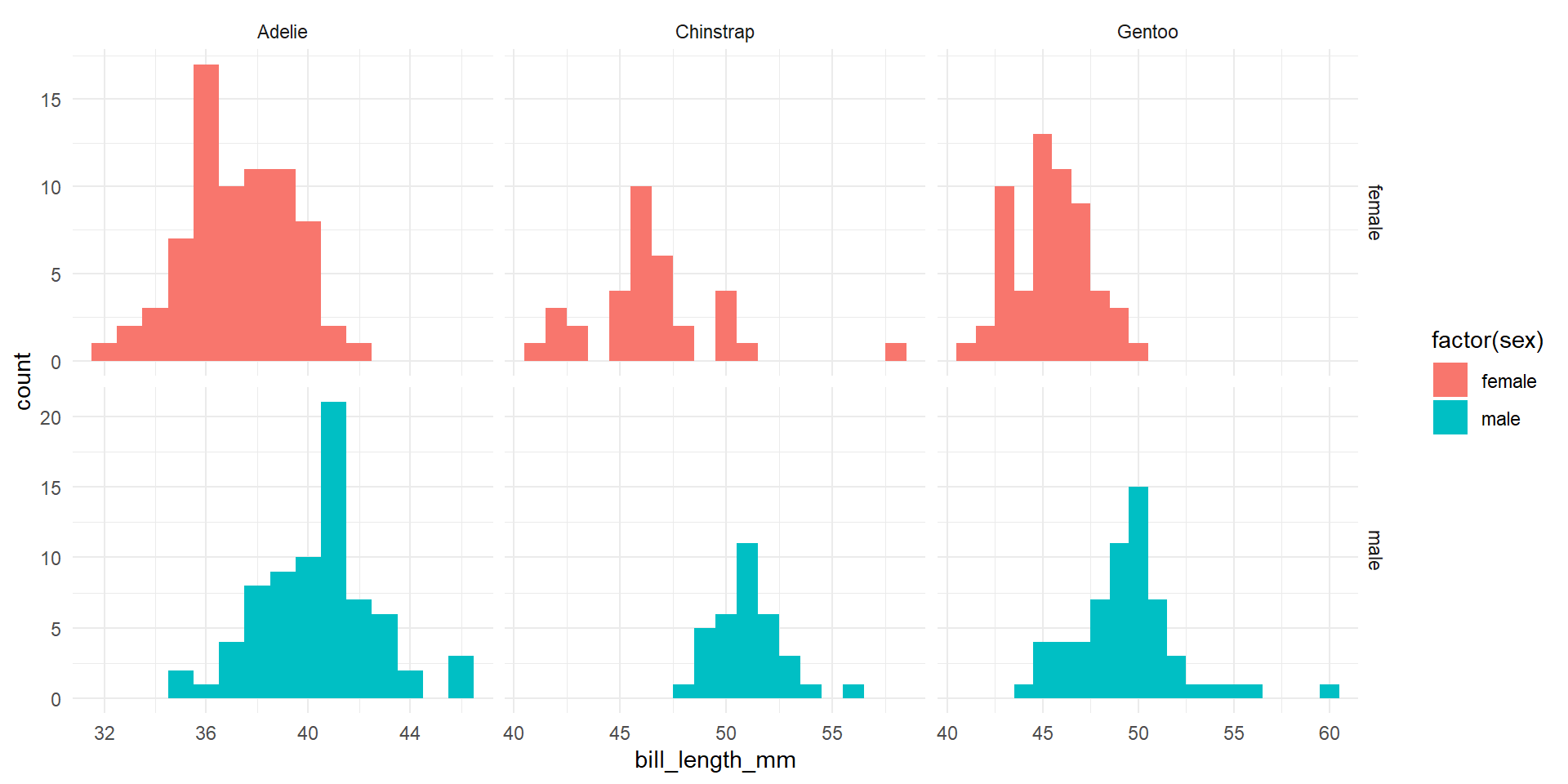
1 female:Adelie 37.3 2.03
2 female:Chinstrap 46.6 3.11
3 female:Gentoo 45.6 2.05
4 male:Adelie 40.4 2.28
5 male:Chinstrap 51.1 1.56
6 male:Gentoo 49.5 2.72A Note for Assumption Checking
Two-Way ANOVA Function
             Df Sum Sq Mean Sq F value Pr(>F)
sex           1   1175    1175 219.228 <2e-16 ***
species       2   6976    3488 650.479 <2e-16 ***
sex:species   2     24      12   2.284  0.103
Residuals   327   1753       5
---
Signif. codes:  0 '***' 0.001 '**' 0.01 '*' 0.05 '.' 0.1 ' ' 1
11 observations deleted due to missingness
Main Effect 2
Interaction Effect
  Tukey multiple comparisons of means
    95% family-wise confidence level

Fit: aov(formula = bill_length_mm ~ sex + species + sex * species, data = penguins)

$`sex:species`
                                     diff       lwr        upr     p adj
male:Adelie-female:Adelie        3.132877  2.034137  4.2316165 0.0000000
female:Chinstrap-female:Adelie   9.315995  7.937732 10.6942588 0.0000000
male:Chinstrap-female:Adelie    13.836583 12.458320 15.2148470 0.0000000
female:Gentoo-female:Adelie      8.306259  7.138639  9.4738788 0.0000000
male:Gentoo-female:Adelie       12.216236 11.064727 13.3677453 0.0000000
female:Chinstrap-male:Adelie     6.183118  4.804855  7.5613821 0.0000000
male:Chinstrap-male:Adelie      10.703707  9.325443 12.0819703 0.0000000
female:Gentoo-male:Adelie        5.173382  4.005762  6.3410021 0.0000000
male:Gentoo-male:Adelie          9.083360  7.931851 10.2348686 0.0000000
male:Chinstrap-female:Chinstrap  4.520588  2.910622  6.1305547 0.0000000
female:Gentoo-female:Chinstrap  -1.009736 -2.443514  0.4240412 0.3338130
male:Gentoo-female:Chinstrap     2.900241  1.479553  4.3209291 0.0000002
female:Gentoo-male:Chinstrap    -5.530325 -6.964102 -4.0965471 0.0000000
male:Gentoo-male:Chinstrap      -1.620347 -3.041035 -0.1996591 0.0149963
male:Gentoo-female:Gentoo        3.909977  2.692570  5.1273846 0.0000000
An Important Note
- When interactions are present, the main effects of factors don’t have their usual interpretations.
- Because of this, we usually test for the presence of interactions first.
- If interactions are present, then we often stop the analysis at this stage and examine interaction effects.
- If no evidence for an interaction effect is found (i.e., if we do not reject \(H_0\)), then we proceed to testing the main effects of the individual factors.
- Because of this, we usually test for the presence of interactions first.
- So in this example, we ignored Main Effect 1 & Main Effect 2 and examine the Interaction Effect!