One-Way Randomized Blocks Design & Introduction to Two-Way ANOVA
STAT 218 - Week 10, Lecture 1
March 11th, 2024
Introduction
In a randomized blocks design,
- We first group the experimental units into sets, or blocks, of relatively similar units
- We randomly allocate treatments within each block.
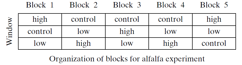
Example: Alfalfa and Acid Rain Researchers were interested in the effect that acid has on the growth rate of alfalfa plants.
- They created three treatment groups (IV) in an experiment: low acid, high acid, and control.
- The response variable (DV) in their experiment was the height of the alfalfa plants in a Styrofoam cup after 5 days of growth.
- They had 5 cups for each of the 3 treatments, for a total of 15 observations.
- However, the cups were arranged near a window and they wanted to account for the effect of differing amounts of sunlight.
- Thus, they created 5 blocks —each block was a fixed distance away from the window (block 1 being the closest through block 5, the farthest).
- However, the cups were arranged near a window and they wanted to account for the effect of differing amounts of sunlight.
- Within each block the three treatments were randomly assigned.
But Why?
In general, we create blocks
- in order to reduce or eliminate variability caused by extraneous variables
- so that the precision of the experiment is increased.
- We want the experimental units within a block to be homogeneous;
- We want the extraneous variability to occur between the blocks.
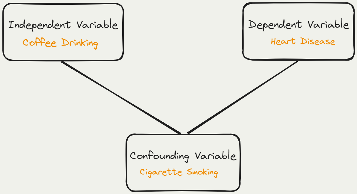
Confounding Variable vs Extraneous Variable
Creating the Blocks
As the preceding examples show, blocking is a way of organizing the inherent variation that exists among experimental units.
Ideally, the blocking should be arranged so as to increase the information available from the experiment.
- To achieve this goal, the experimenter should try to create blocks that are as homogeneous within themselves as possible so that the inherent variation between experimental units becomes, as far as possible, variation between blocks rather than within blocks
Another Example for Blocking
Blocking in an Agricultural Field Study
When comparing several varieties of grain, an agronomist will generally plant many field plots of each variety and measure the yield of each plot.
Differences in yields may reflect not only genuine differences among the varieties, but also differences among the plots in soil fertility, pH, water-holding capacity, and so on.
- Consequently, the spatial arrangement of the plots in the field is important.
An efficient way to use the available field area is
- to divide the field into large regions—the blocks—and
- to subdivide each block into several plots.
- Within each block the various varieties of grain are then randomly allocated to the plots, with a separate randomization done for each block.
- For instance, suppose we want to test four varieties of barley.
- Then each block would contain four plots.
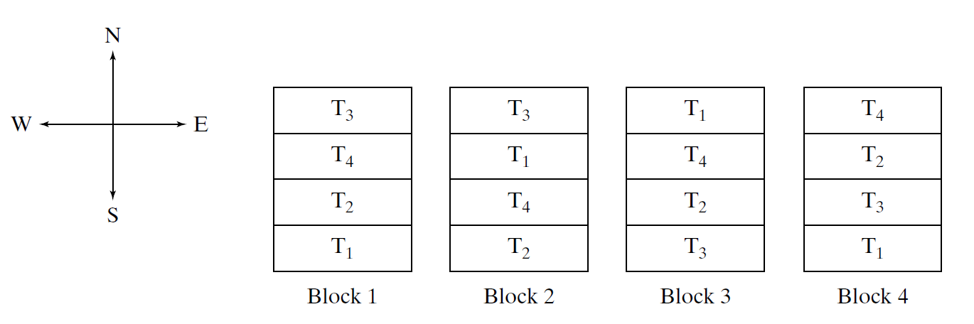
- The resulting randomized allocation might look like Figure 11.6.2, which is a schematic map of the field.
- The “treatments” \(T_1\), \(T_2\), \(T_3\), and \(T_4\) are the four varieties of barley.
- For instance, suppose we want to test four varieties of barley.
The Randomization Procedure
Once the blocks have been created, the blocked allocation of experimental units is straightforward:
- It is as if a mini-experiment is conducted within each block.
- Randomization is carried out for each block separately,
Agricultural Field Study (cont.d)
Consider the agricultural field experiment of Example 11.6.4.
- In block 1, let us label the plots 1, 2, 3, 4, from north to south (see Figure 11.6.2); we will allocate one plot to each variety.
- The allocation proceeds as for the completely randomized design, by choosing plots at random from the four, and assigning the first plot chosen to \(T_1\), the second to \(T_2\), and so on.
- For instance, using a computer to randomly permute the numbers 1 through 4 (or even shuffled cards numbered 1 through 4) we might obtain the sequence 4, 3, 1, 2, which would lead to the following treatment allocation.
| Block 1 | |
|---|---|
| T1 | Plot 4 |
| T2 | Plot 3 |
| T3 | Plot 1 |
| T4 | Plot 2 |
- This is in fact the assignment shown in Figure 11.6.2 for block 1. We can then repeat this procedure for blocks 2, 3, and so on.
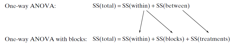
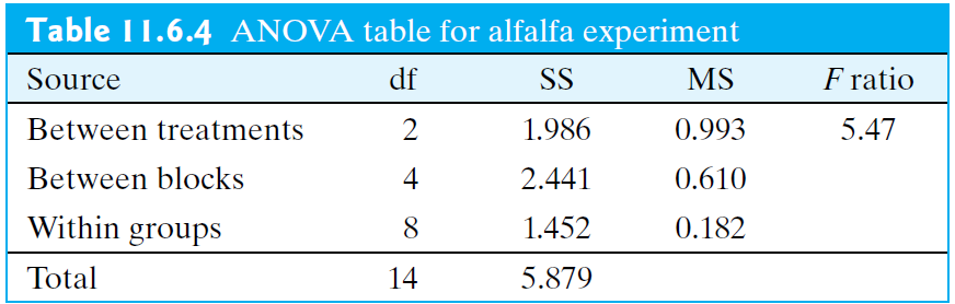
Analyzing Data from a Randomized Block Experiment
In the same way we cannot use a two-sample t test when data are paired, when an experiment has been blocked, we no longer can use our ANOVA methods that we learned in Section 11.4.
- Instead, we will use a randomized blocks ANOVA model.(You are not responsible to calculate \(F\) statistic for this)
Analyzing Data from a Randomized Block Experiment