The Chi-Square for Goodness of Fit & The Chi-Square Test for Independence

STAT 218 - Week 7, Lecture 3 Lab 6

February 22^th, 2024

What is Chi-Square Test?

The chi-square distribution is sometimes used to characterize data sets and statistics that are always positive and typically right skewed.
The chi- square distribution has just one parameter called degrees of freedom (\(df\)), just like in the \(t\)-test which influences the shape, center, and spread of the distribution.
- Recall a normal distribution had two parameters - mean (\(\mu\)) and standard deviation (\(\sigma\))

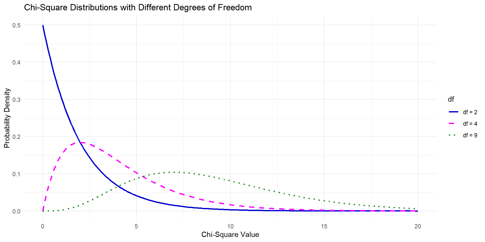
Example of Some Chi-Square Disributions

As the degrees of freedom increases:

The distribution becomes more symmetric,
The center moves to the right, and
The variability inflates

When do we need to use this test?

This is commonly used in these circumstances:

Given a sample of cases that can be classified into several groups, determine if the sample is representative of the general population.
Evaluate whether data resemble a particular distribution, such as a normal distribution.
It compares the frequency of cases found in the various categories of one variable across the different categories of another variable.
- In other words, it explores the relationship between categorical variables.

What type of variable(s) do we need to conduct this test?

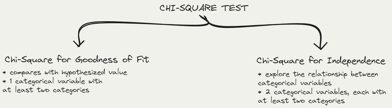
Chi-Square for Goodness of Fit

Introduction

This technique is commonly used in two circumstances:

Given a sample of cases that can be classified into several groups, determine if the sample is representative of the general population.
Evaluate whether data resemble a particular distribution, such as a normal distribution.

What You Need is…

One categorical variable, with two or more categories:
- options (a) and (b) in GSS survey
A hypothesized proportion
- 0.20 selecting (a); 0.80 selecting (b)

Research Question and Data Set

Research Question: Do these data provide convincing evidence that more than 80% of Americans have a good intuition about experimental design?

gss <- data.frame(
  Category = c("All 1000 get the drug", 
               "500 get the drug 500 don't"),
  n = c(99, 571)
)
print(gss)

                    Category   n
1      All 1000 get the drug  99
2 500 get the drug 500 don't 571

Step 1. Formulate Hypotheses

Null Hypothesis (\(H_0\)): The proportion of Americans with a good intuition about experimental design does not differ significantly from 0.80.

Alternative Hypothesis (\(H_A\)): The proportion of Americans with a good intuition about experimental design differs significantly from 0.80.

Step 2. Checking Conditions/Assumptions:

Assumptions

There are two conditions that must be checked before performing a chi-square test:

Independence. Each case that contributes a count to the table must be independent of all the other cases in the table.
Sample size / distribution. Each particular scenario (i.e. cell count) must have at least 5 expected cases.
- IMPORTANT!: We will check this assumption after computing Chi-square statistic
df > 1: Degrees of freedom must be greater than 1.

Failing to check conditions may affect the test’s error rates.

Step 3. Calculate Chi-square statistic and interpret the output.

gss_observed <- c(99, 571)
expected_proportions <- c(0.2, 0.8)
chisquare_gof <- chisq.test(gss_observed, p = expected_proportions)
chisquare_gof


    Chi-squared test for given probabilities

data:  gss_observed
X-squared = 11.427, df = 1, p-value = 0.0007238

Go back to Step 2. Checking Conditions/Assumptions:

Check expected counts for each cell.

chisquare_gof$observed

[1]  99 571

chisquare_gof$expected

[1] 134 536

Step 4. Draw a Conclusion!

Tip

A p-value above .10 (little or no evidence against the null hypothesis.)
A p-value below .10 but above .05 (moderate evidence against the null hypothesis.)
A p-value between .01 and .05 (strong evidence against the null hypothesis - most people consider this convincing.)
A p-value below .01 (very strong evidence against the null hypothesis.)

Reject the null hypothesis

Since the p-value is low (\(p\)-value = 0.0007), we have a very strong evidence against the null hypothesis.

The data provide convincing evidence that the proportion of Americans with a good intuition about experimental design is different than 0.80.

Chi Square Test for Independence

Introduction

It compares the frequency of cases found in the various categories of one variable across the different categories of another variable.

In other words, it explores the relationship between categorical variables.

Is the proportion of smokers to non-smokers the same for males and females?
Are males more likely than females to be smokers?

Warning

A one-way table describes counts for each outcome in a single variable. A two-way table describes counts for combinations of outcomes for two variables. When we consider a two-way table, we often would like to know, are these variables related in any way? That is, are they dependent (versus independent)?

What You Need is…

2 categorical variables, each with at least two categories.
- Level of concern: “A great deal” vs. “Not a great deal”
- Groups: “Duke Students” vs. “US Residents”

Research Question and Data Set

Research Question: Do these data suggest that the proportion of all Duke students who would be concerned a great deal by the melting of the northern ice cap differs from the proportion of all Americans who do?

# We create a 2 by 2 table
table_data <- matrix(c(69, 36, 454, 226), nrow = 2)

# We convert it to a data frame
concern_gw <- as.data.frame(table_data)

# We add meaningful column and row names
colnames(concern_gw) <- c("Duke", "US")
rownames(concern_gw) <- c("A Great Deal", "Not A Great Deal")

print(concern_gw)

                 Duke  US
A Great Deal       69 454
Not A Great Deal   36 226

Step 1 Formulate Hypotheses

\(H_0\) = The proportion of Duke students who concerned about global warming is the same as the proportion of US residents.

\(H_A\) = The proportion of Duke students who concerned about global warming is not the same as the proportion of US residents.