Inference for Categorical Data
STAT 218 - Week 7, Lecture 2
February 21th, 2024
Inference For A Single Proportion
Sampling Distribution and Conditions
Sampling Distribution of \(\hat{p}\)
The sampling proportion for \(\hat{p}\) based on a sample size \(n\) from a population with a true proportion \(p\) is nearly normal when
- the observations are independent e.g., are from a simple random sample
- at least 10 successes and 10 failures in the sample, i.e. \(np \geq 10\) and \(n(1-p) \geq 10\). We call this success-failure condition.
When these conditions/assumptions are met, then the sampling distribution of \(\hat{p}\) is nearly normal with mean \(p\) and the standard error equal to
\[ SE = \sqrt{\frac{p(1-p)}{n}} \]
\(p\) = Population proportion
\(\hat{p}\) = Sample proportion
Be Careful!
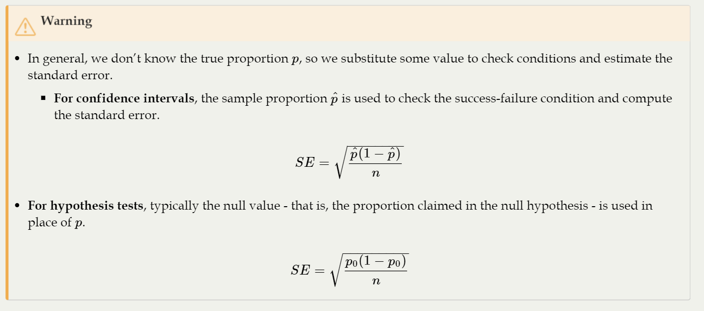
Confidence Intervals for a Proportion
A confidence interval provides a range of plausible values for the parameter \(p\), and when \(\hat{p}\) can be modeled using a normal distribution, the confidence interval for \(p\) takes the form
\[ \hat{p} \pm z^{\ast} \times SE_{\hat{p}} \]
Motivating Example - I
Two scientists want to know if a certain drug is effective against high blood pressure.
The first scientist wants to give the drug to 1000 people with high blood pressure and see how many of them experience lower blood pressure levels.
The second scientist wants to give the drug to 500 people with high blood pressure, and not give the drug to another 500 people with high blood pressure, and see how many in both groups experience lower blood pressure levels.
Which is the better way to test this drug?
- All 1000 get the drug
- 500 get the drug, 500 don’t
Motivating Example - II
We would like to estimate the proportion of all Americans who have good intuition about experimental design, i.e. would answer “500 get the drug 500 don’t”?
In the 2010 survey, it is found that 571 out of 670 (85%) of Americans answered the question on experimental design correctly (the sample was randomly chosen).
- What are the parameter of interest and the point estimate?
Parameter of interest: proportion of all Americans \(p\) who have good intuition about experimental design.
Point estimate: proportion of sampled Americans (\(\hat{p}\)) who have good intuition about experimental design.
Motivating Example - CI
Estimate (using a 95% confidence interval) the proportion of all Americans who have good intuition about experimental design.
- Check Conditions/Assumptions
- Calculate the Standard Error of a sample proportion
- Calculate 95% Confidence Interval
- (0.82, 0.88)
Hypothesis Testing for a Proportion
- Let’s use the same example.
- The 2010 survey found that 571 out of 670 (85%) of Americans answered the question on experimental design correctly.
- Do these data provide convincing evidence that more than 80% of Americans have a good intuition about experimental design?
\(H_0: p = 0.80\)
\(H_A: p >0.80\) (one tailed)
Hypothesis Testing for a Proportion
Remember!
\[ SE = \sqrt{\frac{p_0 (1-p_0)}{n}} \] \[ SE = \sqrt{\frac{0.80 \times 0.20}{679}} = 0.0154 \]
\[ Z = {\frac{0.85 - 0.80}{0.0154}} = 3.25 \] Let’s check the Table 4.
\(p\) value = 1-0.9994 = 0.0006.
What would be our decision?
When one or more conditions aren’t met
What happens when the success-failure condition fails? What about when the independence condition fails?
- In either case, the general ideas of confidence intervals and hypothesis tests remain the same, but the strategy or technique used to generate the interval or p-value change.
When the success-failure condition isn’t met for a hypothesis test,
- we can simulate the null distribution of \(\hat{p}\) using the null value, \(p_0\).
For a confidence interval when the success-failure condition isn’t met,
- we can use what’s called the Clopper-Pearson interval. The details are beyond the scope of this course.
The independence condition is a more nuanced requirement. When it isn’t met, it is important to understand how and why it isn’t met.
Difference of Two Proportions
Introduction
Sampling Distribution of \(\hat{p_1}\) - \(\hat{p_2}\)
We can extend what we have learned.
The differences in population proportions for \(\hat{p_1} - \hat{p_2}\) can be modeled using a normal distribution when
- The data are independent within and between the two groups.
- Generally this is satisfied if the data come from two independent random samples or if the data come from a randomized experiment.
- The success-failure condition holds for both groups, where we check successes and failures in each group separately.
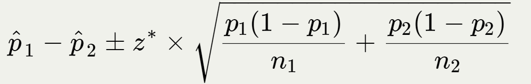
When these conditions/assumptions are met, then the standard error of \(\hat{p_1} - \hat{p_2}\) is equal to
\[ SE = \sqrt{\frac{p_1(1-p_1)}{n_1} + \frac{p_2(1-p_2)}{n_2}} \] where \(p_1\) and \(p_2\) represent the population proportions, and \(n_1\) and \(n_2\) represent the sample sizes.
Confidence Intervals for a \(p_1\) - \(p_2\)
We can apply the generic confidence interval formula for a difference of two proportions
An Example - I
Scientists predict that global warming may have big effects on the polar regions within the next 100 years. One of the possible effects is that the northern ice cap may completely melt.
Would this bother you a great deal, some, a little, or not at all if it actually happened?
- A great deal
- Some
- A little
- Not at all
Motivating Example - II
The GSS asks the same question, below are the distributions of responses from the 2010 GSS as well as from a group of introductory statistics students at Duke University:
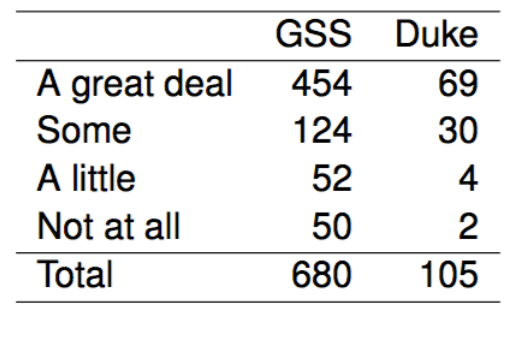
Parameter of interest: Difference between the proportions of all Duke students and all Americans who would be bothered a great deal by the northern ice cap completely melting.
Point estimate: Difference between the proportions of sampled Duke students and sampled Americans who would be bothered a great deal by the northern ice cap completely melting.
An Example - CI
Construct a 95% confidence interval for the difference between the proportions of Duke students and Americans who would be bothered a great deal by the melting of the northern ice cap (\(p_{Duke}\) - \(p_{US}\)).
- Check Conditions/Assumptions
- Calculate the Standard Error of a sample proportion
- Calculate 95% Confidence Interval
- 95% CI = (-0.108, 0.086)
- I’ll leave this as an exercise.