Inference for a Single Proportion

STAT 218 - Week 7, Lecture 1

February 20^th, 2024

Announcements

• Grace days
  • Leave a comment on Canvas instead of emailing
• Determining your data set
  • Check the instructions, please!
• Determining Variables
  • Deadline is today!
• Rendering issue
  • You should see me during my office hours. You will not be able to upload just .qmd file beginning from this week
• Final Exam Date and Time
  • Sat, Mar 16 at 10:15 AM (2 hours) at BLDG 008-0123

Last Week’s Glossary - Check Your Understanding!

na.omit()	infer package	t_test()	facet_wrap(~group)
Ancymidol	Student’s t distribution	Independent samples t test	Hypothesis Testing
Paired sample t test	degrees of freedom	Oceano Dunes State Park	false positive
false negative	Type I Error`	Type II Error	Power
Null Hypothesis	Alternative Hypothesis	Higgs boson	One-tailed test
Two-tailed test	Decision Error	Checking Assumptions	One sample t test

Today’s Menu

• The goals of this weeks are
  • to introduce the logic of inference for a categorical variable (Tue)
    • to state the null and alternative hypotheses in words and in terms of the symbols.
    • to explain how to conduct a simulation using a null hypotheses probability that is not 50-50.
    • to calculate confidence interval
  • to apply confidence intervals and hypothesis tests to differences in population proportions (Wed)
  • to introduce testing for goodness of fit using chi-square (Thu)
  • to introduce testing for independence in two-way tables (Thu)

Today’s activity will be based on one of the resources of STUB – Statistical Thinking in Undergraduate Biology

Let’s Refresh Our Memory

We will scaffold today’s content with those previous knowledge

• Probability: the long-run frequency/proportion of times an outcome occurs in repeated trials under identical conditions
• Key terminology: observational unit, variable, statistic, sample, parameter, population
• Data Summarization: shape, center, spread
  
• 68/95/99.8 rule: With bell-shaped distributions, approximately 95% of observations fall within 2 Standard Deviation of mean

Motivating Example

Dogs have a keen sense of smell. They are used for search and rescue, explosive detection, sniffing out illegal drugs in luggage at airports, and locating game while hunting.

• Can they also tell whether someone has COVID-19 by sniffing a specimen of sweat from a person?

We will be looking at a study that used several dogs to test this question.

• We will focus on one dog, Maika, a 3-year-old female Belgian Malinois whose specialty is search and rescue.
  • Maika completed 57 trials where she would sniff four different sweat specimens, one of which was from a COVID positive person, and then sit in front of the specimen she determined to be the positive specimen.

• The researchers found that in 47 of the 57 trials Maika chose the COVID positive specimen.

Let’s identify the observational unit, type of variable, statistic, sample, parameter, and population.

Motivating Example

• Let’s produce a bar graph representing the observed results.

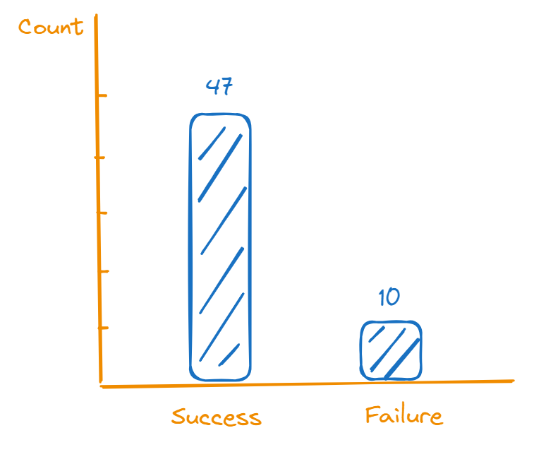
• Do these results convince you that dogs can detect COVID-19?

• How many would Maika need to get correct to convince you?
  • Does it need to be all 57?
• If Maika does not have some ability to identify the COVID specimen from the sweat of a person, what is another explanation for her getting so many correct?
• Research Question?
  • Does Maika tend to correctly identify the COVID specimen?

Motivating Example

• There are two possible explanations for this tendency:
  • In the long-run, Maika has a genuine tendency to correctly identify the COVID specimen
    
  • In the long run, Maika does not have a genuine tendency and is simply guessing among the specimen each time (she got lucky)
    
• Suppose a friend thinks Maika just got lucky (Is that null hypothesis or alternative hypothesis?).
  • How could you convince your friend otherwise? OR
  • How likely do you think it is that Maika was able to identify so many correctly if she was simply guessing each time.
• Let’s suggest a method and map it!

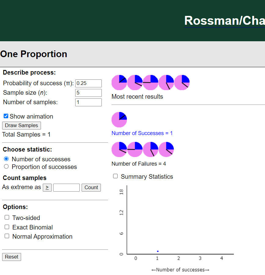
One Proportion Using A Spinner

• Let’s use our applet to generate “null distribution”.

Steps To Be Followed:

We will draw multiple samples and simulate data to observe the number of successes.

Your Turn:

• Set the probability of success as 0.25
  
• Set the sample size as 5
• Observe what happens if you draw only 1 sample.
  
• Record the number of success
  
• Did everyone in class obtained the same result for their guessing dog?
  • Let’s compile those results in a dotplot
    • What are the observational units in this graph?
    • What is the variable in this graph?

My Turn:

• Set the probability of success as 0.25
  
• Set the sample size as 57
• Observe what happens if you draw 100 samples.
  
• Keep pressing “Draw Samples” until the distribution stops changing much
  
• Interpret the graph.

Formulate Conclusions

• Based on these simulation results, would you consider it surprising for Maika to correctly identify the COVID specimen 47 times?

• Let’s reconsider those two competing explanations. Which one appears more plausible to you?
  • In the long-run, Maika has a genuine tendency to correctly identify the COVID specimen
  • In the long run, Maika does not have a genuine tendency and is simply guessing among the specimens each time (she got lucky)
• In this case, the observed statistic is far out in the tail of the distribution and it is not hard to see that Maika’s proportion of successful identifications is unlikely to happen by random chance.

Some questions before you go…

• Do you consider the observed sample result to be statistically significant?
  • Recall that this means that the observed result is unlikely to have occurred by chance alone.
• How broadly are you willing to generalize your conclusions?
  • Would you be willing to generalize your conclusions to all dogs? Explain your reasoning.

Hypothesis Testing - Strength of Evidence against the null hypothesis

Attempt to estimate the interval for the p-value in today’s motivating example with a different approach.

• A p-value above .10 (little or no evidence against the null hypothesis.)

• A p-value below .10 but above .05 (moderate evidence against the null hypothesis.)

• A p-value between .01 and .05 (strong evidence against the null hypothesis - most people consider this convincing.)

• A p-value below .01 (very strong evidence against the null hypothesis.)

Note

Remember our binary decision that we did last week! (if \(p \leq \alpha\), then reject \(H_0\))

• Which option appears more comprehensive?