Ch. 7 & Ch. 8: Applications of \(t\)-tests
STAT 218 - Week 6, Lecture 3 Lab 4
February 14th, 2024
What Have We Learned So Far?
A Snapshot
- Descriptive Statistics describes and summarizes data.
- Includes understanding
- distribution shape (skewed, normal, etc.),
- central tendency (mean, median, mode), and
- spread (variance, standard deviation, range).
- Includes understanding
- Inferential Statistics makes predictions and draws conclusions about populations based on sample data.
- We saw different types of t-tests:
- One sample t-test: compares a sample mean to a known or hypothesized population mean.
- Independent samples t-test: compares means of two independent groups.
- Paired samples t-test: compares means of two related groups or one group with two different measurements/occasions.
- We saw different types of t-tests:
Estimation and Hypothesis Testing
We learned that we can estimate the unknown parameters in two ways:
Point estimation: A single value calculated from the sample (e.g., \(\bar{y}\))
Confidence Intervals: A range of values within which the parameter is expected to fall, with a certain degree of confidence.(e.g., 95% CI, 90% CI)
We also learned that we can use hypothesis testing to test for a specific value(s) of the parameter.
- e.g., \(H_0: \mu = 76\) cm & \(H_A: \mu \neq 76\) cm (Two-tailed test)
- \(H_0: \mu_1 - \mu_2 = 0\) cm \(H_A: \mu_1 > \mu_2\) (One-tailed test)
Hypothesis Testing Steps
Revising the Steps of Hypothesis Testing and \(p\)-values
Important
Last lecture, we had 4 steps
- Construct the Hypotheses of \(H_0\) and \(H_A\)
- Determine your \(\alpha\) level
- Calculate test statistic and find the P-value
- Draw conclusion.
Revising the Steps of Hypothesis Testing and \(p\)-values
Important
Today, we will add one more step to these lab sessions
- Construct the Hypotheses of \(H_0\) and \(H_A\)
- Determine your \(\alpha\) level
- Check the assumptions
- Compute test statistic and find the P-value (Interpreting R Output)
- Draw conclusion.
Assumptions - Verification of Conditions
- It is always important to check first whether the conditions are reasonable in a given case.
- Here is the list of assumptions that we should be aware of for \(t\)-tests.
1) Random Sampling: the data can be regarded as coming from independently chosen random sample(s),
2) Independence of Observations: the observations should be independent within each sample, and
3) Normal Distribution: Many of the methods depend on the data being from a population that has a normal distribution.
- REMEMBER! If sample size is large, then condition (3) is less important (Central Limit Theorem).
Normality Assumption - I
If the only source of information is the data at hand, then normality can be roughly checked by making a histogram and normal quantile plot of the data.
- Unfortunately, for a small or moderate sample size, this check is fairly rudimentary.
- If the sample is large, then the visual plots give us good information about the population shape;
- However, if \(n\) is large, the requirement of normality is less important anyway due to the Central Limit Theorem.
In any case, a rudimentary check is better than none, and every data analysis should begin with inspection of a graph of the data, with special attention to any observations that lie very far from the center of the distribution.
Normality Assumption - II
We check assumptions before conducting any statistical analysis. To check normality assumption, we need to first check sample size.
\(1^{st}\) option - small samples: Check the \(p\)-value of Shapiro Wilk test. It is best used with a sample size less than 50 (Shapiro & Wilk 1965; Uttley,2019).
\(2^{nd}\) option - large samples: Check the visual plots (e.g., histogram, normal quantile plot) if your sample size is more than 50.
One Sample \(t\)-test
To-Do List
- Download the worksheet and dataset from the course website.
- Save them to your STAT 218 folder (VERY IMPORTANT).
Introduction
- In one sample \(t\) tests, data collected from one sample and compares the mean score with a test value.
- Test value can be
- reported previously in the literature; or
- found by calculating level of chance.
- Test value can be
- In this example, we will work with the several data sets. To begin with, we need
inferpackage to conduct t tests. - Let’s load that package by using
install.packages()function.
Introduction
Example of a Case:
Imagine that you are a biologist studying penguins, particularly their bill lengths. You hypothesize that the average bill length of penguins is 40 mm and you collect a random sample of 344 penguins, measure and record their bill length in mm.
Perform a one sample \(t\)-test to investigate whether the bill length of the penguins differs from the test value of 40 mm. Use the 5% significance level (\(\alpha = 0.05\)).
Checking the Normality Assumption
- Check your sample size first!
- \(n\) > 50, so we can check visual plots.
Quantile Plot
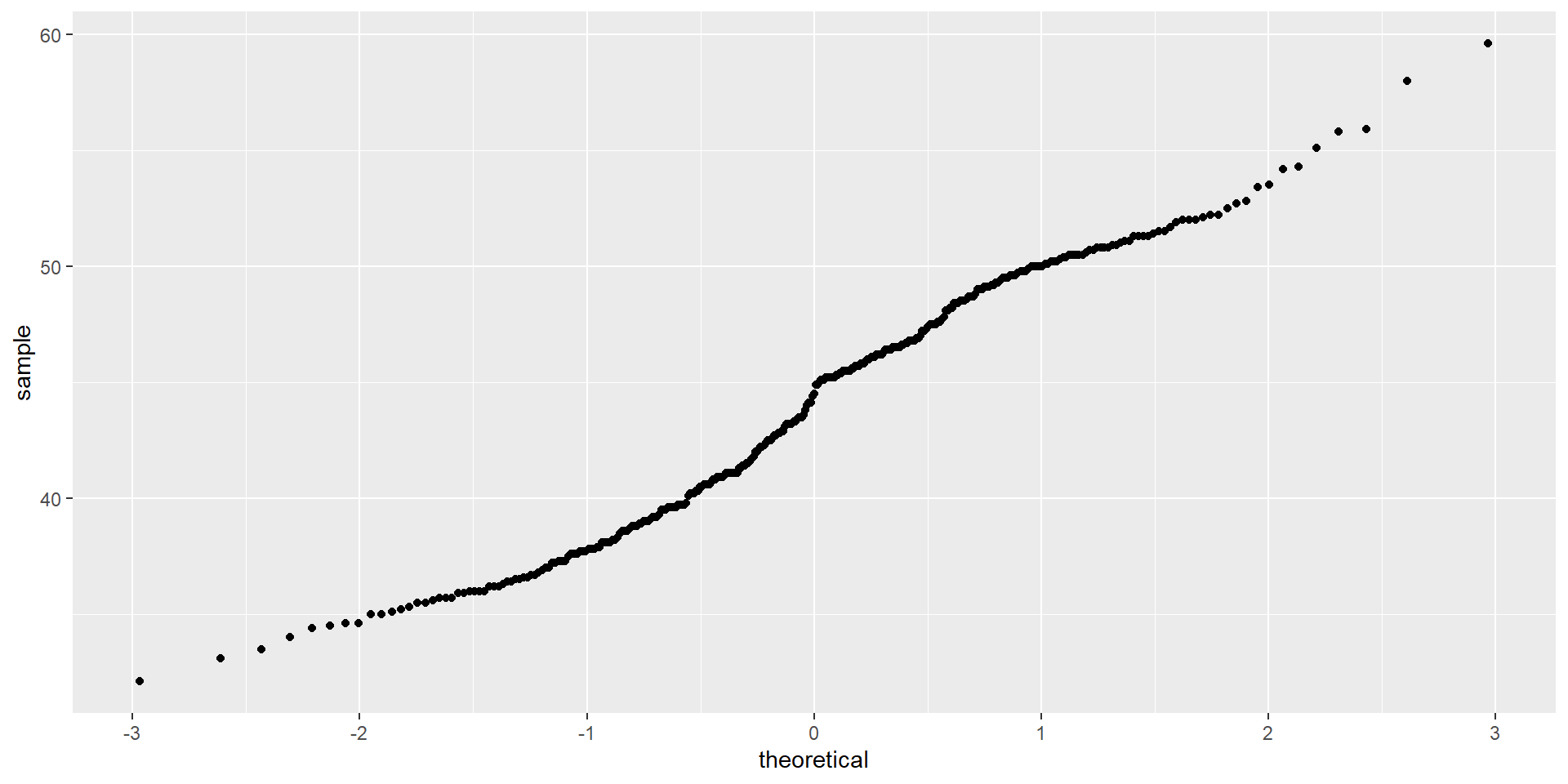
Interpreting the Output
# A tibble: 1 × 7
  statistic  t_df  p_value alternative estimate lower_ci upper_ci
      <dbl> <dbl>    <dbl> <chr>          <dbl>    <dbl>    <dbl>
1      13.3   341 9.58e-33 two.sided       43.9     43.3     44.5
Conclusion: As \(P\)-value is very small, we can reject \(H_0\) and conclude that our data provided sufficient evidence to support the claim that the bill length of the penguins differs from 40 mm.
Confidence Interval: Type your confidence interval statement to your worksheet!
Independent Samples \(t\)-test
Introduction
- Independent samples \(t\) test compares means of two independent groups.
- 1 DV (numeric) + 1 IV(categorical)
- Your IV should have 2 groups (e.g., male, female)
Example of a Case:
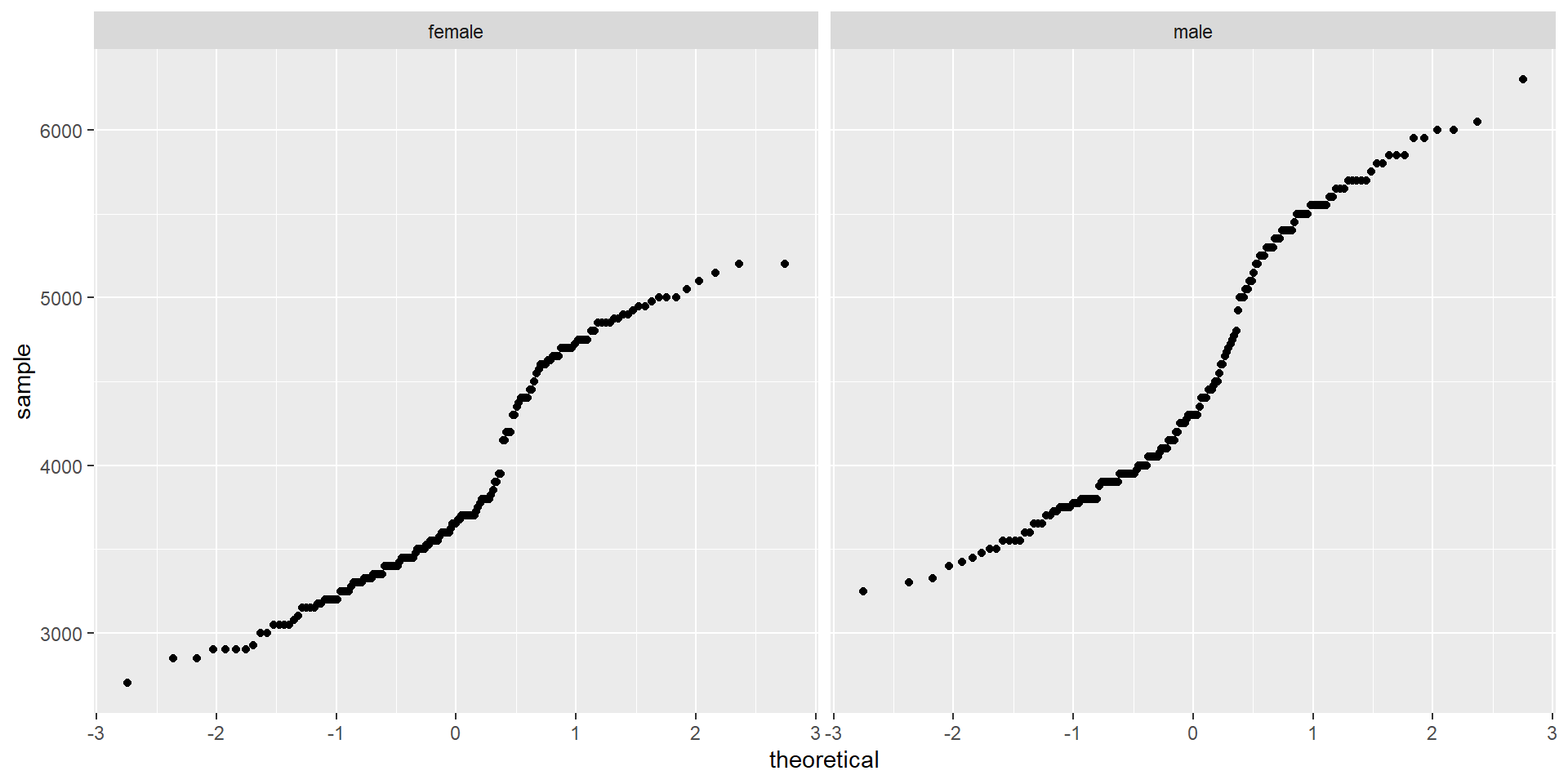
Now, you’re curious about the difference in the body mass of penguins based on their sex. You hypothesize that body mass varies between different sexes. To test your hypothesis, you collect a random sample of 344 penguins, measure their body mass, and record their sex.
Perform an independent samples \(t\)-test to investigate whether the body mass of penguins differs between different sexes. Use the 10% significance level (\(\alpha = 0.10\)).
Checking the Normality Assumption
- Check your sample size first!
- \(n\) > 50, so we can check visual plots.
Quantile Plots
Interpreting the Output
t_test(x = penguins,
       formula = body_mass_g ~ sex,
       order = c("male", "female"),
       alternative = "two-sided",
       conf_level = 0.90)
# A tibble: 1 × 7
statistic t_df p_value alternative estimate lower_ci upper_ci
<dbl> <dbl> <dbl> <chr> <dbl> <dbl> <dbl>
1 8.55 324. 4.79e-16 two.sided 683. 552. 815.Conclusion: Type your conclusion statement to your worksheet!
Confidence Interval: Type your confidence interval statement to your worksheet!
Paired Samples \(t\)-test
Introduction
- Paired samples \(t\) test compares means of two related groups or one group with two different measurements/occasions.
- 1 DV (numeric) + 1 IV(categorical)
- Your IV should be two related groups or one group with two different measurements/occasions.
Example of a Case: Pollutants in a stream may accumulate or attenuate as water flows down the stream. In a study to monitor the accumulation and attenuation of fecal contamination in a stream running through cattle rangeland, monthly water specimens were collected at two locations along the stream over a period of 21 months.
The data set stream the total coliform count (MPN/100ml) for a water specimen.
Perform a paired samples \(t\)-test to assess whether the mean total coliform count is consistent across the two locations. Use the 5% significance level (\(\alpha = 0.05\)).
Checking the Normality Assumption
- Check your sample size first!
- \(n\) < 50, so we should check Shapiro-Wilk test.
- \(n\) < 50, so we should check Shapiro-Wilk test.
- This output is from a calculation of Shapiro-Wilk test. We generally use Shapiro-Wilk test for relatively smaller sample size because visuals can be misleading in smaller sample sizes. Please interpret Shapiro-Wilk \(p\)-value.
Shapiro-Wilk normality test
data: stream$Difference W = 0.9641, p-value = 0.6022
Interpreting the Output
# A tibble: 1 × 7
  statistic  t_df  p_value alternative estimate lower_ci upper_ci
      <dbl> <dbl>    <dbl> <chr>          <dbl>    <dbl>    <dbl>
1      4.61    20 0.000170 two.sided      1103.     604.    1602.
Conclusion: Type your conclusion statement to your worksheet!
Confidence Interval: Type your confidence interval statement to your worksheet!