One Sample \(t\)-tests & Comparison of Paired Samples

STAT 218 - Week 6, Lecture 1

February 12^th, 2024

Hypothesis Testing

What is Hypothesis Testing?

Important

NULL AND ALTERNATIVE HYPOTHESES

• The null hypothesis (\(H_0\)) often represents a skeptical perspective or a claim to be tested.
  
• The alternative hypothesis (\(H_A\)) represents an alternative claim under consideration and is often represented by a range of possible parameter values.
• Our job as life scientists is to play the role of a skeptic: before we buy into the alternative hypothesis, we need to see strong supporting evidence.

A Hypothesis Testing Example From Physics

In 2012, physicists suggested that they had discovered the existence of a subatomic particle known as the Higgs boson, based on some data and a \(P\)-value of 0.0000003. What they meant was:

• If the particle does not exist (the null hypothesis), then the probability of their data (or more extreme) was 0.0000003. That is a lot less than the arbitrary 0.05 and is pretty convincing.

One-tailed vs Two tailed tests

A two-tailed test is used to test the null hypothesis against the alternative hypothesis which is also known as nondirectional alternative. \[ \\H_0: \mu_1 = \mu_2 \\H_A: \mu_1 \neq \mu_2 \]

In some studies it is apparent from the beginning—before the data are collected— that there is only one reasonable direction of deviation from \(H_0\). In such situations it is appropriate to formulate a directional alternative hypothesis. \[ \\H_0: \mu_1 = \mu_2 \\H_A: \mu_1 < \mu_2 \] OR

\[ \\H_0: \mu_1 = \mu_2 \\H_A: \mu_1 > \mu_2 \]

Hypothesis Testing Steps

Introduction

The general idea is to formulate as a hypothesis the statement and then to see whether the data provide sufficient evidence.

Important

We have 4 steps to do that

1. Construct the Hypotheses of \(H_0\) and \(H_A\)
2. Determine your \(\alpha\) level
3. Calculate test statistic and find the p-value
4. Draw conclusion.

One Sample \(t\)-tests

Introduction

• In one sample \(t\) tests, data collected from one sample and compares the mean score with a test value.
  • Test value can be
    
  1. reported previously in the literature; or
     
  2. found by calculating level of chance.

Example

The average time for all runners who finished the Cherry Blossom Race in 2006 was 93.29 minutes (93 minutes and about 17 seconds). We want to determine using data from 100 participants in the 2017 Cherry Blossom Race whether runners in this race are getting faster or slower, versus the other possibility that there has been no change.

The sample mean and sample standard deviation of the sample of 100 runners from the 2017 Cherry Blossom Race are 97.32 and 16.98 minutes, respectively.(\(\alpha = 0.05\))

\(H_0\): The average 10-mile run time was the same for 2006 and 2017.
\(\mu\) = 93.29 minutes.

\(H_A\): The average 10-mile run time for 2017 was different than that of 2006. \(\mu \neq 93.29\) minutes.

Example (Cont.d)

\[ SE = s/ \sqrt{n} \\ 16.98 \sqrt{100} = 1.70 \]

\[ t_s = \frac {{97.32 - 93.29}}{1.70} = 2.37 \]

for \(df = 100 - 1 = 99\), we can find the \(P\)-value by using computer as \(P\)-value = 0.02

Conclusion: Because the \(P\)-value is smaller than 0.05, we reject the null hypothesis. That is, the data provide strong evidence that the average run time for the Cherry Blossom Run in 2017 is different than the 2006 average.

Comparison of Paired Samples

Introduction

When do we need to use this test?

• 1 group, 2 different occasions or under 2 different conditions (pre-test/post-test)

• Matched subjects

Notation

In this paired-sample \(t\) test we analyze differences

\[ D = Y_1 - Y_2 \] Then \(\bar{D}\) can be considered as follows:

\[ \bar{D} = \bar{Y_1} - \bar{Y_2} \]

which can be an analogous of

\[ \mu_D = {\mu_1} - {\mu_2} \] We may say that the mean of the difference is equal to the difference of the means.

Example 8.1.1

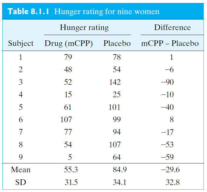
Hunger Rating During a weight loss study, each of nine subjects was given (1) the active drug m-chlorophenylpiperazine (mCPP) for 2 weeks and then a placebo for another 2 weeks, or (2) the placebo for the first 2 weeks and then mCPP for the second 2 weeks. As part of the study, the subjects were asked to rate how hungry there were at the end of each 2-week period.

Let us test \(H_0\) against \(H_A\) at significance level \(\alpha\) = 0.05.

\(H_0: \mu_{D} = 0\) \(H_A: \mu_{D} \neq 0\)

Example 8.1.1.

\[ SE_{\bar{D}} = \frac{s_D}{\sqrt{n_D}} \]

\[ t_s= \frac {\bar{d} - \mu_{D}}{SE_{\bar{D}}} \]

\[ SE_{\bar{D}} = \frac{32.8}{\sqrt{9}} = 10.9 \]

\[ t_s= \frac {-29.6 - 0}{10.9} = -2.71 \] Using a computer gives the \(P\)-value as \(P\)= 0.027.

Reject \(H_0\) and find that there is sufficient evidence to conclude that hunger when taking mCPP is different from hunger when taking a placebo.

Decision Errors

An Introduction to Decision Errors

Type I Error (\(\alpha\))

Definition

\(\alpha\) = Pr{finding significant evidence for \(H_A\)} if \(H_0\) is true

OR

rejecting the null hypothesis when \(H_0\) is actually true.

• Claiming that data provide evidence that significantly supports \(H_A\) when \(H_0\) is true is called a Type I error.
• In choosing (\(\alpha\)), we are choosing our level of protection against Type I error.
  • Many researchers regard 5% as an acceptably small risk.
    • If we do not regard 5% as small enough, we might choose to use a more conservative value of a such as a = 0.01; in this case the percentage of true null hypotheses that we reject would be not 5% but 1%.
• In practice, the choice of a may depend on the context of the particular experiment.
  • A regulatory agency might demand more exacting proof of efficacy for a toxic drug than for a relatively innocuous one.
• Also, a person’s choice of (\(\alpha\)) may be influenced by his or her prior opinion about the phenomenon under study.
  • Suppose an agronomist is skeptical of claims for a certain soil treatment; in evaluating a new study of the treatment, he might express his skepticism by choosing a very conservative significance level (say, (\(\alpha\)) = 0.001), thus indicating that it would take a lot of evidence to convince him that the treatment is effective.
  • For this reason, written reports of an investigation should include a \(P\)-value so that each reader is free to choose his or her own value of a in evaluating the reported results.

Type II Error (\(\beta\))

Definition

\(\beta\) = Pr{lack of significant evidence for \(H_A\)} if \(H_A\) is true

OR

failing to reject the null hypothesis when the alternative is actually true.

• If \(H_A\) is true, but we do not observe sufficient evidence to support \(H_A\), then we have made a Type II error.
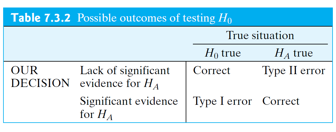
• Table 7.3.2 displays the situations in which Type I and Type II errors can occur.

• For example, if we find significant evidence for \(H_A\), then we eliminate the possibility of a Type II error, but by rejecting \(H_0\) we may have made a Type I error.

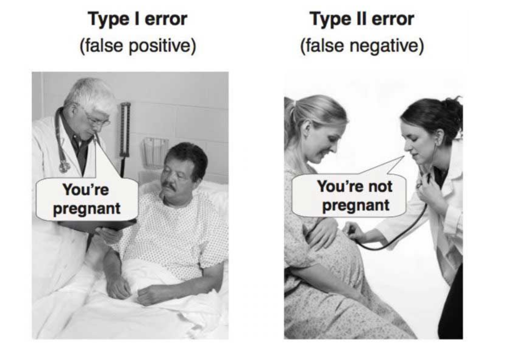
Type I Error vs Type II Error

From Essential Guide to Effect Sizes by Paul D. Ellis (2010)

Power

The chance of not making a Type II error when \(H_A\) is true —that is, the chance of having significant evidence for \(H_A\) when \(H_A\) is true— is called the power of a statistical test:

Definition

Power = 1 - \(\beta\) = Pr{significant evidence for \(H_A\)} if HA is true

• Thus, the power of a \(t\) test is a measure of the sensitivity of the test, or the ability of the test procedure to detect a difference between \(\mu_1\) and \(\mu_2\) when such a difference really does exist.

• In this way the power is analogous to the resolving power of a microscope.

• The power of a statistical test depends on many factors in an investigationincluding

  • the sample sizes,
  • the inherent variability of the observations, and
  • the magnitude of the difference between \(\mu_1\) and \(\mu_2\).

• All other things being equal, using larger samples gives more information and thereby increases power.

Consequences of Inappropriate Use of Student’s t

Our discussion of the t test and confidence interval (in Sections 7.3–7.8) was based on the conditions of

1. the data can be regarded as coming from two independently chosen random samples,

2. the observations are independent within each sample, and

3. each of the populations is normally distributed (If n1 and n2 are large, this condition is less important).

• Violation of the conditions may render the methods inappropriate.
• If the conditions are not satisfied, then the \(t\) test may be inappropriate in two possible ways:

1. It may be invalid in the sense that the actual risk of Type I error is larger than the nominal significance level a. (To put this another way, the \(P\)-value yielded by the \(t\) test procedure may be inappropriately small.)

2. The \(t\) test may be valid, but less powerful than a more appropriate test.

• If the design includes hierarchical structures that are ignored in the analysis, the \(t\) test may be seriously invalid. If the samples are not independent of each other, the usual consequence is a loss of power.