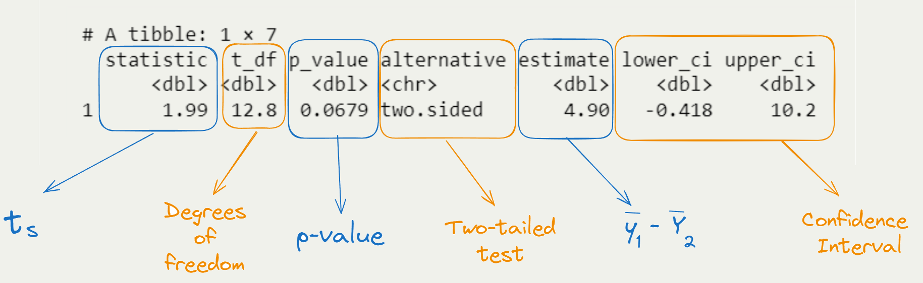
Introduction to Hypothesis Testing & Comparison of Independent Samples

STAT 218 - Week 5, Lecture 4

February 8th, 2024

Introduction to Hypothesis Testing

Setting the Scene

Suppose that we have 2 samples from two populations.

  • If the two samples look quite similar to each other, we might infer that the two populations are identical;

  • If the samples look quite different, we would infer that the populations differ.

  • The question is, then…

    • “How different do two samples have to be in order for us to infer that the populations that generated them are actually different?

An approach: Compare the two sample means to be able to explore how much they differ in comparison to the amount of difference we would expect to see due to chance.

  • We can construct 2 competing ideas.

What is Hypothesis Testing?

Let’s consider this example. We’re interested in understanding how much people know about world health and development. If we take a multiple choice world health question, then we might like to understand if

  • \(H_0\): People never learn these particular topics and their responses are simply equivalent to random guesses.
  • \(H_A\): People have knowledge that helps them do better than random guessing, or perhaps, they have false knowledge that leads them to actually do worse than random guessing.

These competing ideas are called hypotheses. We call \(H_0\) the null hypothesis and \(H_A\) the alternative hypothesis.

Important

NULL AND ALTERNATIVE HYPOTHESES

  • The null hypothesis (\(H_0\)) often represents a skeptical perspective or a claim to be tested.
  • The alternative hypothesis (\(H_A\)) represents an alternative claim under consideration and is often represented by a range of possible parameter values.
  • Our job as life scientists is to play the role of a skeptic: before we buy into the alternative hypothesis, we need to see strong supporting evidence.

Hypothesis Testing for the Difference of (\(\mu_1\) - \(\mu_2\))

Introduction

The general idea is to formulate as a hypothesis the statement that \(\mu_1\) and \(\mu_2\) differ and then to see whether the data provide sufficient evidence in support of that hypothesis.

Important

We have 4 steps to do that

  1. Construct the Hypotheses of \(H_0\) and \(H_A\)
  2. Determine your \(\alpha\) level
  3. Calculate test statistic and find the P-value
  4. Draw conclusion.

Step 1. The Null and Alternative Hypotheses

The hypothesis that \(\mu_1\) and \(\mu_2\) are not equal is called an alternative hypothesis (or a research hypothesis)

\[ H_A: \mu_1 \neq \mu_2 \]

Its antithesis is the null hypothesis, \[ H_0: \mu_1 = \mu_2 \]

which asserts that \(\mu_1\) and \(\mu_2\) are equal. A researcher would usually express these hypotheses more informally and we can trace those hypotheses from the examples, problems and exercises in this course.

Alternatively we can express these hypotheses as following:

\[ \\H_0: \mu_1 - \mu_2 = 0 \\H_A: \mu_1 - \mu_2 \neq 0 \]

Step 2. Determine your \(\alpha\) level

  • Making a decision requires drawing a definite line between sufficient and insufficient evidence.
  • The threshold value, on the P-value scale, is called the significance level of the test and is denoted by the Greek letter \(\alpha\) (alpha).
  • The value of a is chosen by whoever is making the decision.
    • Common choices are \(alpha\) = 0.10, 0.05, and 0.01.
  • Usually, we will find this information within our example questions.

Step 3. Calculate test statistic and find the P-value

  • The \(t\) test is a standard method of choosing between these two hypotheses. To carry out the \(t\) test, the first step is to compute the test statistic.

  • It is a measure of how far the difference between the sample means (\(\bar{y}\)’s) is from the difference we would expect to see if \(H_0\) were true (zero difference), expressed in relation to the SE of the difference — the amount of variation we expect to see in differences of means from random samples.

  • The subscript “s” on \(t_s\) serves as a reminder that this value is calculated from the data (“s” for “sample”).

  • The quantity \(t_s\) is the test statistic for the \(t\) test; that is, ts provides the data summary that is the basis for the test procedure.

\[ t_s = \frac{(\bar{y}_1 - \bar{y}_2) - (\mu_1 - \mu_2)}{SE(\bar{y}_1 - \bar{y}_2)} \]

Step 3. Calculate test statistic and find the P-value (cont.d)

Step 4. Draw Conclusion

  • Not an easy task. Where does one draw the line in determining how much evidence is sufficient? Most people would agree that
    • P-value = 0.0001 indicates very strong evidence
    • P-value = 0.80 indicates a lack of evidence
    • but what about intermediate values?
  • For example, should P-value = 0.10 be regarded as sufficient evidence for \(H_A\)?
    • The answer is not intuitively obvious.
  • In much scientific research, it is not necessary to draw a sharp line. However, in many situations a decision must be reached.
    • The Food and Drug Administration (FDA) must decide whether the data submitted by a pharmaceutical manufacturer are sufficient to justify approval of a medication.
    • Fertilizer manufacturer must decide whether the evidence favoring a new fertilizer is sufficient to justify the expense of further research.

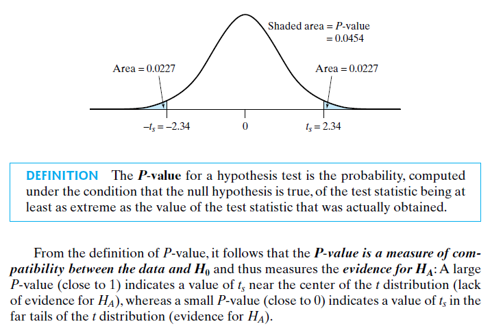
Step 4. Draw Conclusion (cont.d)

Important

We can think of a as a preset threshold of statistical significance (OR the risk of false positive finding).

  • If the P-value of the data is less than or equal to \(\alpha\),
    • the data are judged to provide statistically significant (some like to express this as ‘statistically discernible’) evidence in favor of \(H_A\); we also may say that \(H_0\) is rejected.
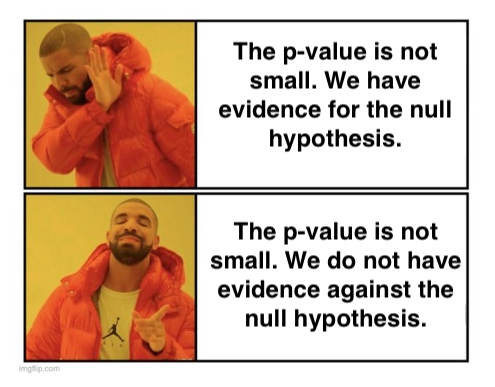
  • If the P-value of the data is greater than \(\alpha\),
    • we can say that the data provide insufficient evidence against the \(H_0\), and thus we fail to reject \(H_0\).

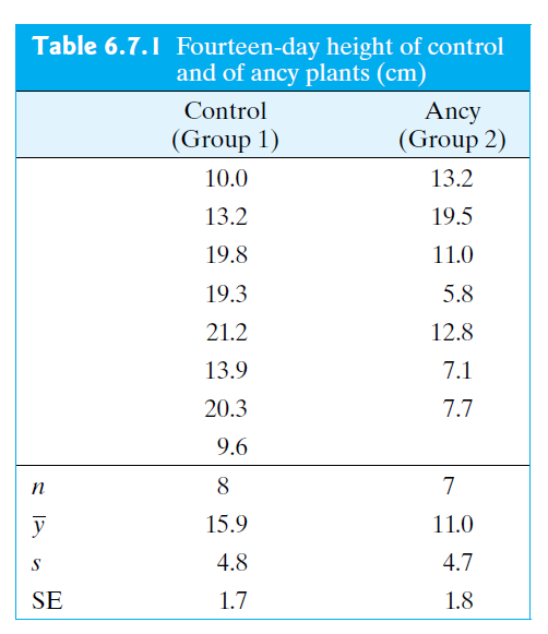
The Same Example for (\(\mu_1\) - \(\mu_2\))

The Wisconsin Fast Plant, Brassica campestris, has a very rapid growth cycle that makes it particularly well suited for the study of factors that affect plant growth.

In one such study, 7 plants were treated with the substance Ancymidol (ancy) and were compared to 8 control plants that were given ordinary water. Heights of all of the plants were measured, in cm, after 14 days of growth.

(\(df\) for this question is calculated as 12).

Let’s see an example for hypothesis testing by using \(\alpha = 0.05\)

R Output

# A tibble: 1 × 7
  statistic  t_df p_value alternative estimate lower_ci upper_ci
      <dbl> <dbl>   <dbl> <chr>          <dbl>    <dbl>    <dbl>
1      1.99  12.8  0.0679 two.sided       4.90   -0.418     10.2

Interpretation of R Output

Assumptions and Validations

Remember!

  1. the data can be regarded as coming from two independently chosen random samples,

  2. the observations are independent within each sample, and

  3. each of the populations is normally distributed.

If \(n_1\) and \(n_2\) are large, condition (3) is less important.