Student’s t Distribution

STAT 218 - Week 5, Lecture 2

February 6^th, 2024

Survey Check-in Before Midterm

Weekly Assignments
- Answer Key
- Feedback
- Grades
Having more practice problems together
RStudio/Coding

Last Week’s Glossary - Check Your Understanding!

`ggplot()`	`babies` data set	`geom_boxplot()`	`geom_bar()`
confidence interval	aesthetics	geometric layer	parity
histogram	binwidth	stacked bar-plot	standardized bar plot
dodged bar plot	boxplot	gestation	Mandatory Paid Vacation
`labs()`	`theme_bw()`	`element_text()`	`geom_point()`

What Did We Learn Last Week?

Confidence Interval for μ
Data Visualization
- Visualizing a Single Categorical Variable
- Visualizing a Single Numeric Variable
- Visualizing Two Categorical Variables
- Visualizing One Categorical and One Numeric Variable
- Visualizing Two Numeric Variables
- Visualizing More Than Two Categories

This week…

We will learn…

Student’s t distribution
Planning a Study to Estimate μ
Comparing two means
Hypothesis Testing and
Independent samples t test

Student’s t distribution

What is t distribution?

\(t\)-distribution is another bell shape and symmetric distribution that can be useful if we do not know anything about population parameters.
The \(t\)-distribution is always centered at zero and has a single parameter: degrees of freedom.
- The shape of the distribution depends on the degrees of freedom.
Broadly speaking, we use \(t\)-distribution with \(df = n − 1\)
- to model the sample mean when the sample size is \(n\).
- As the \(df\) is increasing, the \(t\)-distribution will look more like the standard normal distribution
  - when the \(df\) is about 30 or more, the \(t\) -distribution is nearly indistinguishable from the normal distribution.

What is t distribution?

Comparison of t and the Standard Normal Distribution

Both are symmetric and bell-shaped but \(t\)-distribution has a larger standard deviation.
The \(t\)-distribution has a single parameter: degrees of freedom.
Standard Normal Distribution has two parameters: \(\mu\) and \(\sigma\).
The tails of \(t\) distributions are thicker than the normal curves,
- observations are more likely to fall beyond two standard deviations from the mean than under the normal distribution.

Calculating Confidence Interval for \(t\)

But First, Let’s Refresh Our Memory

For a sample of observations on a quantitative variable Y
- \(\bar{y}\) is an estimate of \(\mu\).
- s is an estimate of \(\sigma\).

We learned that our estimates are subject to sampling error.

Sampling Error: the amount of discrepancy between \(\bar{y}\) and \(\mu\) is described (in a probability sense) by the sampling distribution of \(\bar{Y}\)

As s is an estimate of \(\sigma\), a natural estimate of \(\sigma / \sqrt{n}\) is \(s/\sqrt{n}\)

The standard error of the mean is defined as follow:

\[ SE_\bar{Y} = \frac{s}{\sqrt{n}} \]

Standard Error

In real life, we don’t know population mean \(\mu\) and population standard deviation \(\sigma\).
- which means that we cannot calculate the standard deviation of sampling distribution.
To overcome this, we can calculate standard error of the mean.
- This strategy tends to work well when we have large data set and we can estimate \(\sigma\) using \(s\) accurately.
- However, the estimate is less precise with smaller samples.

How to Read Table 4

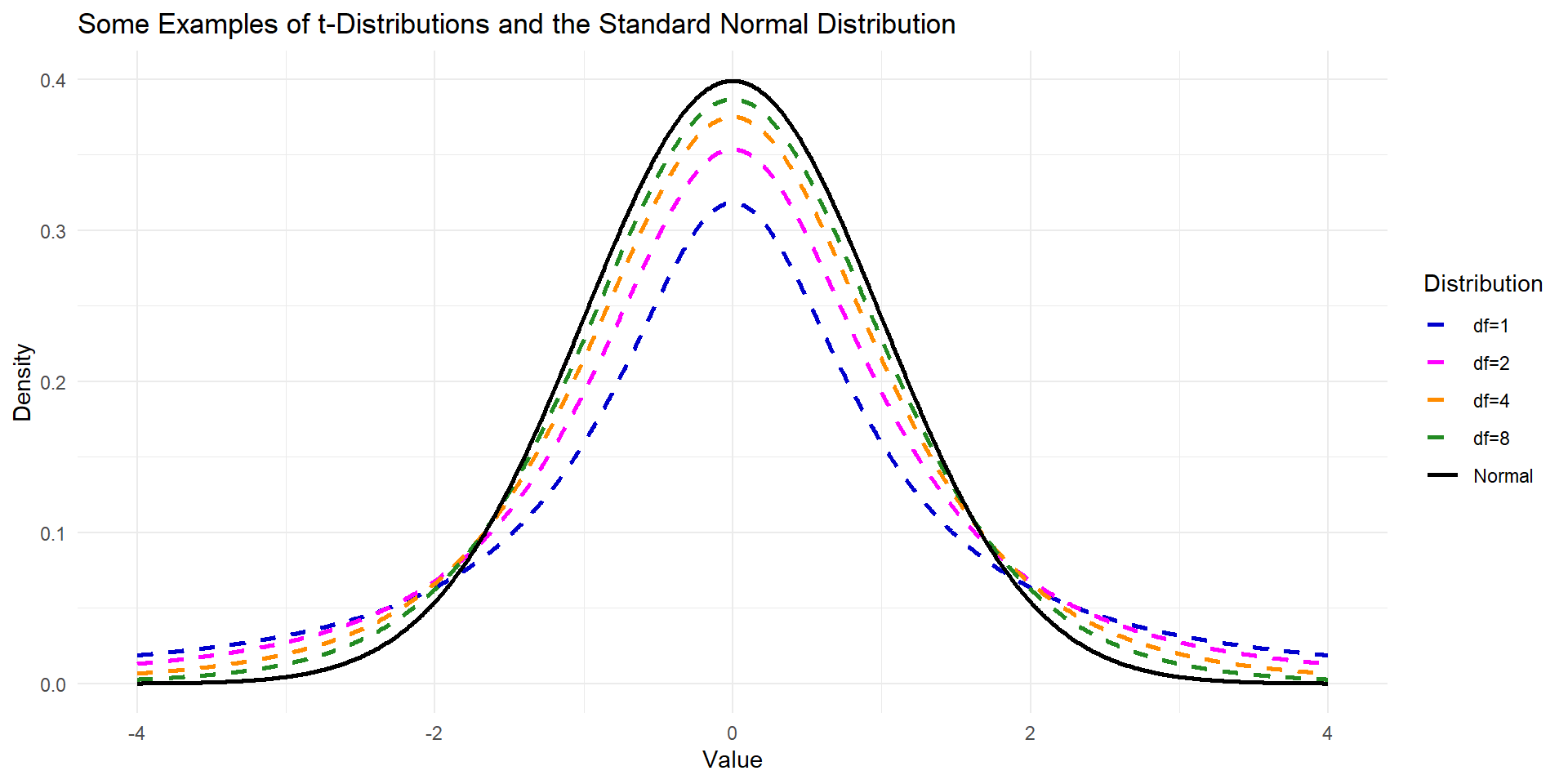
Let’s check Table 4 in our book and see how \(t_{0.025}\) value decreases as the \(df\) increases.
- for \(df = \infty\), the value is \(t_{0.025} = 1.960\) which means that it approached the same value in Table 3 (\(Z\) Scale)

Confidence Interval for t

Last week, we only learned how to calculate 95% CI when we know \(\sigma\)

\[ 95 \% \ CI = (\bar{Y} \pm 1.96 \times \frac{\sigma}{\sqrt{n}}) \]

Now, we will convert this formula to be compatible with \(t\)-distribution \[ 95 \% \ CI = (\bar{y} \pm t_{0.025} \ \times \ SE_{\bar{y}}) \] where

\[ SE_{\bar{y}} = \frac{s}{\sqrt{n}} \]

where the critical value \(t_{0.025}\) is determined from Student’s \(t\)-distribution with

\[ df = n - 1 \]

Same Example from Last Week - I

Let’s have a look wing areas of 14 male Monarch butterflies at Oceano Dunes State Park in California

\(\bar{y} = 32.8143 \ cm^2\) and \(s= 2.4757 \ cm^2\)

Suppose we consider these 14 observations as a random sample from a population.

\[ df = n - 1 \\ df = 14 - 1 \\ df = 13 \]

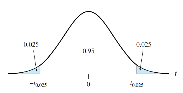
From the Table 4, we find

\[ t_{0.025} = 2.160 \]

Same Example from Last Week - II

95% confidence interval (CI) for \(\mu\) can be calculated as following:

\(\bar{y} = 32.8143 \ cm^2\) and \(s= 2.4757 \ cm^2\)

\[ \\95 \% \ CI = (\bar{y} \pm t_{0.025} \ \times \ SE_{\bar{y}}) \\95 \% \ CI = (32.8143 \pm 2.160 \ \times \ 2.4757 / \sqrt{14}) \]

\[ \\= 32.81 \pm 1.43 \\ 31.43 \ cm^2 < \mu < 34.2 \ cm^2 \\ OR \\ 95 \% \ CI = (31.43,34.2) \]

We are 95% confident that the true population mean is in this confidence interval.

Same Example from Last Week - III

90% confidence interval (CI) for \(\mu\) can be calculated as following:

\(\bar{y} = 32.8143 \ cm^2\) and \(s= 2.4757 \ cm^2\)

\[ \\90 \% \ CI = (\bar{y} \pm t_{0.05} SE_{\bar{y}}) \\90 \% \ CI = (32.8143 \pm 1.771 \ \times \ 2.4757 / \sqrt{14}) \]

\[ \\= 32.81 \pm 1.17 \\ 31.64 \ cm^2 < \mu < 33.98 \ cm^2 \]

We are 90% confident that the true population mean is in this confidence interval.

Think-pair-share: What is the difference between 90% CI and 95% CI?

Planning a Study to Estimate μ

Before collecting data for a research study, it is wise to consider in advance whether the estimates generated from the data will be sufficiently precise.
- It can be painful indeed to discover after a long and expensive study that the standard errors are so large that the primary questions addressed by the study cannot be answered.
The precision with which a population mean can be estimated is determined by two factors:

the population variability of the observed variable Y, and
the sample size.

Planning a Study to Estimate μ

In some situations the variability of Y cannot, and perhaps should not, be reduced.
- For example, a wildlife ecologist may wish to conduct a field study of a natural population of fish; the heterogeneity of the population is not controllable and in fact is a proper subject of investigation.
On the other hand, it is often appropriate, especially in comparative studies, to reduce the variability of Y by holding extraneous conditions as constant as possible.
- For example, physiological measurements may be taken at a fixed time of day; tissue may be held at a controlled temperature; all animals used in an experiment may be the same age

What sample size will be needed?

Recall that

\[ SE_{\bar{y}} = \frac{s}{\sqrt{n}} \]

We can use this formula to determine our sample size as follows:

\[ Desired \ SE = \frac{Guessed \ SD}{\sqrt{n}} \]

Same Example from Last Week - IV

Suppose the researcher is now planning a new study of butterflies Monarch butterflies at Oceano Dunes State Park in California and has decided that it would be desirable that the SE be no more than \(0.4 \ cm^2\)

\(\bar{y} = 32.8143 \ cm^2\) and \(s= 2.4757 \ cm^2\)

\[ SE_{\bar{y}} = s / \sqrt{n} \]

\[ Desired \ SE = Guessed \ SD / \sqrt{n} \]

\[ \\Desired \ SE = 2.48 / \sqrt{n} \ \le 0.4 \\ n\ge 38.4 \] \[ \\ at \ least \ 39 \ butterflies \]

You may wonder how a researcher would arrive at a value such as \(0.4 \ cm^2\) for the desired SE. Such a value is determined by considering how much error one is willing to tolerate in the estimate of μ.

Conditions for Validity of Estimation Methods - I

Note

1. Conditions on the design of the study

(a) It must be reasonable to regard the data as a random sample from a large population.

(b) The observations in the sample must be independent of each other.

2. Conditions on the form of the population distribution

(a) If \(n\) is small, the population distribution must be approximately normal.

(b) If \(n\) is large, the population distribution need not be approximately normal. The requirement that the data are a random sample is the most important condition.

Conditions for Validity of Estimation Methods - II

If the only source of information is the data at hand, then normality can be roughly checked by making a histogram and normal quantile plot of the data if your sample size is large.
- However, if \(n\) is large, the requirement of normality is less important anyway.
Sometimes a histogram or normal quantile plot of the data indicates that the data did not come from a normal population.
- If the sample size is small, then Student’s \(t\)-method will not give valid results.
  - However, it may be possible to transform the data to achieve approximate normality and then analyze the data in the transformed scale.