Ch 6: Confidence Interval

STAT 218 - Week 4, Lecture 2

February 5^th, 2024

Some Announcements

• Quiz answer keys are available on Canvas
  
• There is an opportunity if you are interested in.
  • Funded summer program in biostatistics and data science
  • Applications due - March 15
    
• Check-in survey before the exam (5 minutes)
  • Go to our Canvas page and participate in the survey (It is under the section of Quizzes)

Central Limit Theorem

Definition

• The Central Limit Theorem states that, no matter what distribution Y may have in the population, if the sample size is large enough, then the sampling distribution of \(\bar{Y}\) will be approximately a normal distribution.

• The significance of the Central Limit Theorem lies in its applicability when the shape of the population distribution is unknown, a common scenario in practical situations.

• How large a sample size is required?

  • For a normal distribution, any \(n\) suffices.
  • For moderately nonnormal distributions, a moderate \(n\) is adequate.
  • For highly nonnormal distributions, a rather large \(n\) becomes necessary.

Comparison of Distributions

Comparison of Distributions

Statistical Estimation

Statistical Estimation

• We assume that our data set is a random sample from some population
  • This assumption enables us to use the information in that sample to infer facts about the population.

• Statistical estimation is a form of statistical inference in which we use the data to
  1. determine an estimate of some feature of the population and
  2. assess the precision of the estimate.

An Example for Statistical Estimation

Let’s have a look wing areas of 14 male Monarch butterflies at Oceano Dunes State Park in California

• \(\bar{y} = 32.81\) \(cm^2\) and \(s= 2.48\) \(cm^2\)

Suppose we consider these 14 observations as a random sample from a population.

• \(\mu\) = the (population) mean wing area of male Monarch butterflies in the Oceano Dunes region
• \(\sigma\) = the (population) SD of wing area of male Monarch butterflies in the Oceano Dunes region

From the sample data we have, we can say that

• 32.81 is an estimate of \(\mu\).
• 2.48 is an estimate of \(\sigma\).

Statistical Estimation cont.d

We should be aware of the fact that these estimates are subject to sampling error.

Warning

• This is NOT measurement error;
  • No matter how accurately each individual butterfly was measured, the sample information is imperfect
    • due to the fact that only 14 butterflies were measured, rather than the entire population of butterflies.

• Broadly speaking, for a sample of observations on a quantitative variable Y
  • \(\bar{y}\) is an estimate of \(\mu\).
  • s is an estimate of \(\sigma\).

And our goal is to estimate \(\mu\).

Standard Error of the Mean

Sampling Error: the amount of discrepancy between \(\bar{y}\) and \(\mu\) is described (in a probability sense) by the sampling distribution of \(\bar{Y}\)

• As s is an estimate of \(\sigma\), a natural estimate of \(\sigma / \sqrt{n}\) is \(s/\sqrt{n}\)

The standard error of the mean is defined as follow:

\[ SE_\bar{Y} = \frac{s}{\sqrt{n}} \]

Standard Error of the Mean cont.d

• SE is an estimate of \(\sigma_\bar{y}\).
  • It can be interpreted in terms of the expected sampling error:
    • In a broader sense, the difference between \(\bar{y}\) and \(\mu\) is rarely more than a few standard errors.
    • Not surprisingly, we expect \(\bar{y}\) to be within about one standard error of \(\mu\).
    • Thus, the smaller the SE, the more precise the estimate.
    • And, sample size is a factor that affect the magnitude of SE
• Remember Example 5.2.2

Standard Error vs Standard Deviation

• These two quantities describe entirely different aspects of the data.
  • The SD describes the dispersion of the data,
  • SE describes the unreliability (due to sampling error) in the mean of the sample.
• As the sample size increases,
  • The sample mean and SD tend to approach more closely the population mean and SD
  • The standard error, by contrast, tends to decrease as n increases; when n is very large, the SE is very small and
    • so the sample mean is a very precise estimate of the population mean.

Confidence Interval

An Introduction to Confidence Interval - I

• Our aim is to…
  • determine an estimate of \(\mu\)
    • \(\bar{y}\) was an estimate of \(\mu\)
• We also know that the difference between \(\bar{y}\) and \(\mu\) is rarely more than a few standard errors.

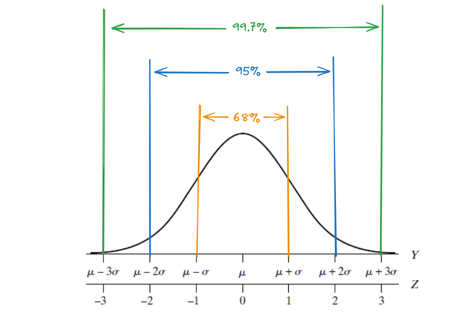
Tip

If \(Z\) is a standard normal random variable, then the probability that \(Z\) is between \(\pm\) 2 is about 0.95 (OR 95% if we remember The 68/95/99.7 rule)

An Introduction to Confidence Interval - II

To understand how to calculate confidence intervals, we need to have

• standardization formula
• standard error
• Z Score Table (Table 3 in our book) and
• solve an equation that composed of these

An Introduction to Confidence Interval - III

• Let’s calculate 95% confidence interval

Tip

If \(Z\) is a standard normal random variable, then the probability that \(Z\) is between \(\pm\) 2 is about 95% (Remember The 68/95/99.7 rule)

\[ Pr\{ -1.96 < \frac{\bar{Y}-\mu}{\sigma/\sqrt{n}} < 1.96 \} =0.95 \]

If you solve this, it will become

\[ 95 \% \ CI = (\bar{Y} \pm 1.96 \sigma / \sqrt{n}) \]

A Further Example from Your Weekly Assignment

Exercise 5.2.8 The heights of a certain population of corn plants follow a normal distribution with mean 145 cm and standard deviation 22 cm. We collected data from 16 plants and calculated the sample mean as 135 cm.

If \(\bar{Y}\) represents the mean height of a random sample of 16 plants from the population (which is 135), 95% confidence interval (CI) for \(\mu\) can be calculated as following:

\[ 95 \% \ CI = (\bar{Y} \pm 1.96 \ X\ \sigma / \sqrt{n}) \]

\[ = (135\pm 1.96 \ X \ 22 / \sqrt{16}) \]

\[ =(124.22,145.78) \]

Understanding Confidence Intervals

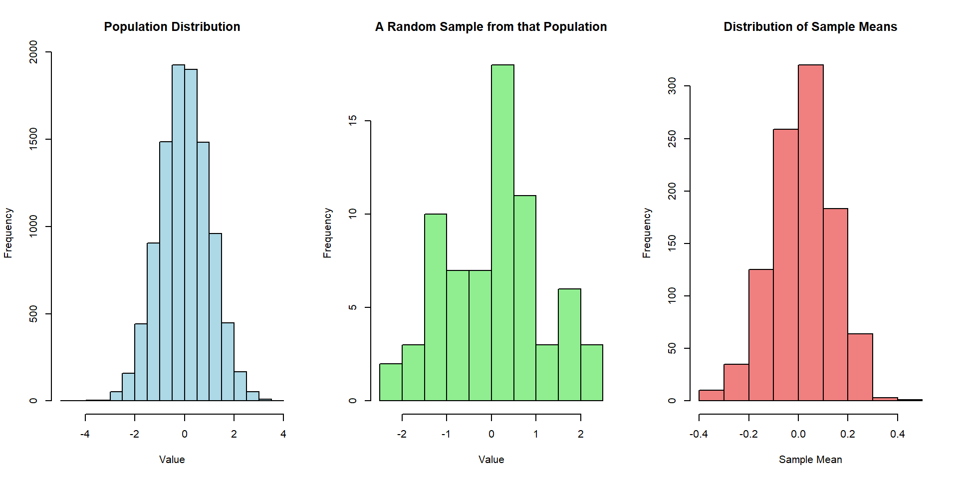
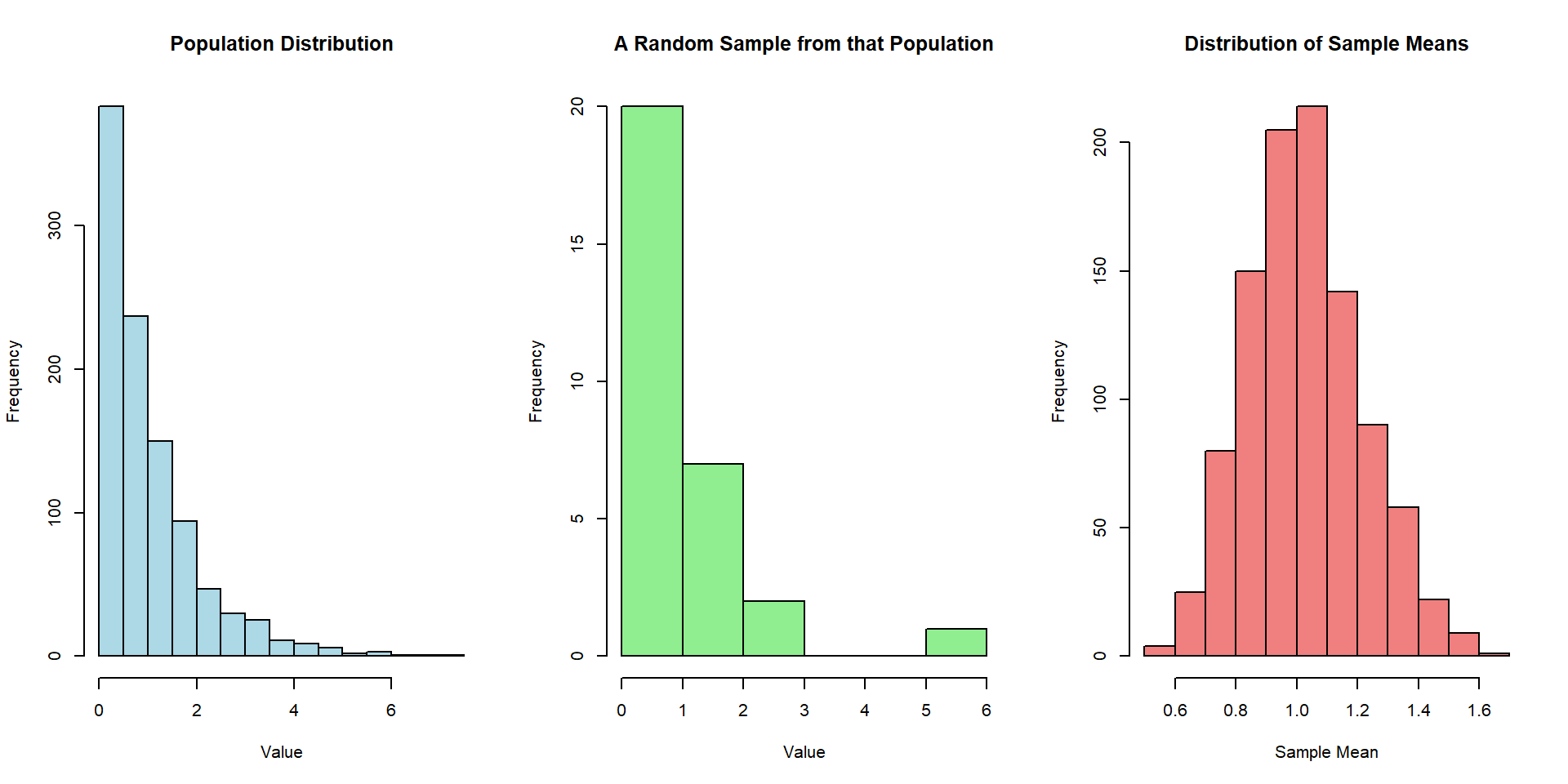
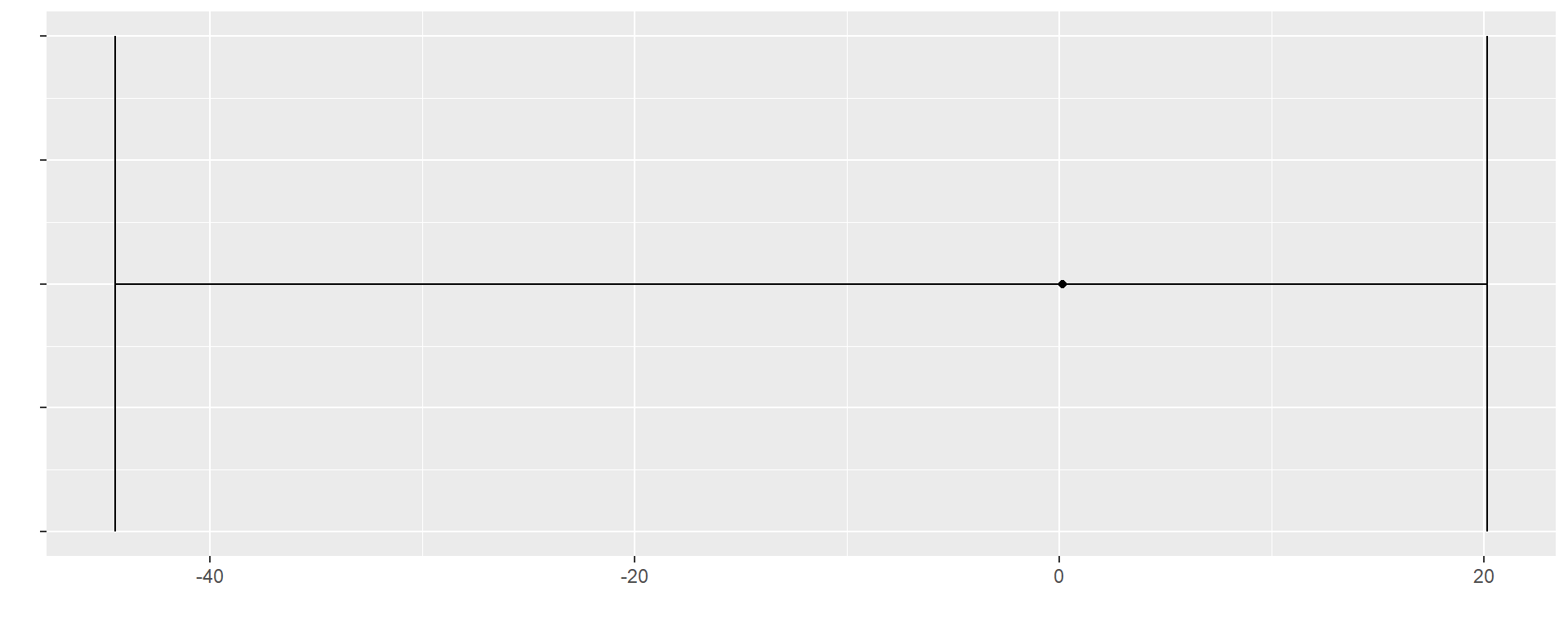
To help you visualize, imagine we have a population, and from that population, we randomly select a group of 20 observational units

95%CI = (-44.47, 20.13)

Understanding Confidence Intervals

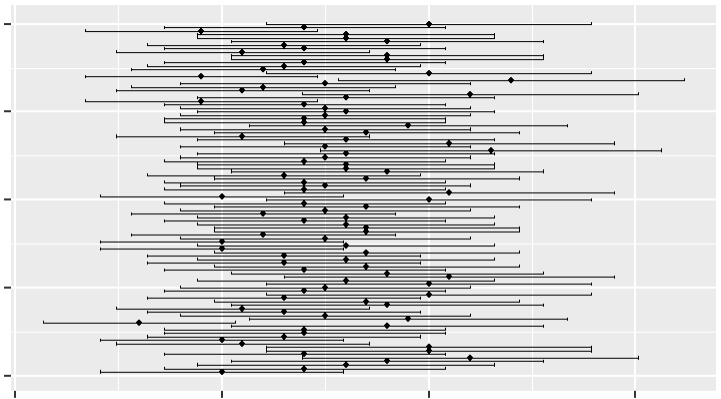
If we repeat this process 100 times, creating 100 different samples of 20 observational units each, we would end up with 100 different samples drawn from the population.

Understanding Confidence Intervals

If we calculate confidence intervals for each of these 100 samples, we will find that…

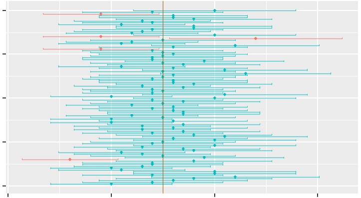
• Around 95% of these intervals capture the true population mean
• We are 95% confident that the true population mean is in this confidence interval.

Confidence Interval - Verbal Explanation

And…

• If we calculate confidence intervals for each of these 100 samples, we will find that around 95% of these intervals capture the true population mean.

• We are 95% confident that the true population mean is in this confidence interval.

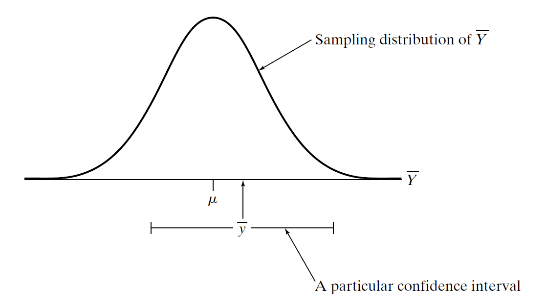
Confidence Interval and Sampling Distribution