An Introduction to Sampling Distribution
STAT 218 - Week 4, Lecture 1
January 29th, 2024
Let’s Refresh Our Memory
Last week we…
- explored the spread of distributions
- reviewed basic concepts of probability
- identified the relationship between probability and the life science
- had an introduction to normal probability distribution
- learned several ways to assess Normality
- performed some summary statistics functions in R
Last Week’s Glossary - Check Your Understanding!
| deviation from the mean | sample standard deviation | sample variance | palmer penguins |
| quartiles | interquartile range (IQR) | outlier | range |
| Normal curve | probability | Normality | love bombing |
| discrete variable | healthy boundaries | density curve | chance |
| robustness | saber-toothed tigers | YAML (what?) | .csv |
| exponential distribution | bimodal | right-skewed | left-skewed |
| standard normal distribution | standardization formula | percentile | within \(\pm\) 1 SD of the mean |
| Normal Quantile Plot | The Shapiro-Wilk test | histogram | The 68/95/99.7 rule |
This week, we will…
- describe the concept of “sampling distribution”.
- identify the relationship between sample size and the accuracy of the sample mean.
- explain the Central Limit Theorem (fingers crossed!)
- calculate Confidence Intervals for µ .
- elaborate on data visualization techniques in R.
- review the topics for Midterm 1.
Introduction
In data analysis, our primary goal as life scientists is to distinguish actual biological features from those that might be the result of random chance.
Generally we obtain a single random sample, which comes from a very large population.
- Today, we will explore the outcomes of selecting:
- a single random sample with the different sample sizes and
- infinitely many random samples with replacement from the same population.
- Then, we will solve a problem which will be very similar with your homework
- Today, we will explore the outcomes of selecting:
Revisiting the Fish Length Example
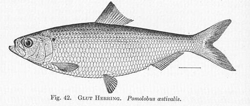
- Please remember the Example 4.3.1 from our course textbook.
Length of Fish: Here is what we know about the shape and population parameters:
- The lengths of the individual fish follow a normal distribution (a symmetric and bell-shaped)
- \(\mu\) = 54.0 mm
- \(\sigma\) = 4.5 mm
- We calculated several percentages of the fish are
- less than 60 mm long (90.82% of the fish)
- more than 51 mm long (74.86% of the fish)
- between 51 and 60 mm long (65.68% of the fish)
- less than 60 mm long (90.82% of the fish)
- Now, our job today is to predict what would happen if we selected random samples with replacement from this fish POPULATION in different scenarios.
Share Your Educated Guess
Scan this QR code and share your educated guess for different sampling scenarios.

Thoughts on the Questions
- The size of your random sample affects the accuracy of your single sample mean.
- There will be some sample values that might surprise you.
- Consider the sample mean as a variable, as you may obtain different sample means in each trial.
- The distribution of all possible sample means tends to have a familiar shape.
Reese Pieces
In the length of fish example, we predicted what would happen in two different scenarios.
Let’s use our applet to see another example regarding proportions.

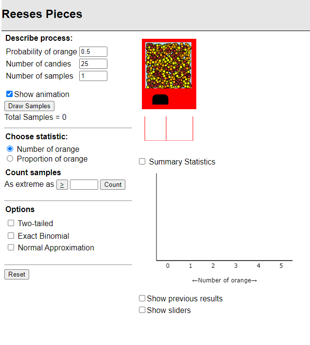
Steps To Be Followed:
We will draw multiple samples of three different sizes and simulate data to observe how it affects the variability of the sample proportions for different sample sizes.
Your Turn:
- Number of Candies is 10
- Set the probability of orange is 0.5
- Fix the number of candies at 10
- Choose statistics as Number of Orange
- Observe what happens if you draw only 1 sample.
- Repeat this 4-5 times.
- Observe what happens if you increase the number of samples to 1,000.
- Click on “Summary Statistics”
- Set the probability of orange is 0.5
My Turn:
- Number of Candies is 10, 25, 1000
- Set the probability of orange is 0.5
- Fix the number of candies as 10, then 25, AND 1000
- Choose statistics as the proportion of orange
- Observe what happens if you have only 1-3 samples.
- Observe what happens if you increase the number of samples to 1,000.
- Use snipping tool to compare the shapes of the distributions.
Take Away Messages
1. In real life, it is impossible to take infinitely many random samples.
Life scientists often work with one single sample.
2. Sample statistics vary from sample to sample.
We see different proportions in each trial.
3. The mean of the all possible sample proportions converges to the population proportion.
We increased the number of samples to 1000 and we saw that the proportion distribution of the all sample proportions converges to the population proportion.
4. Sample size is important.
We tested different sample sizes and we observed the as we increase sample size, the standard deviation tends to decrease.
Fish Length Example
We can apply these take away messages to the fish length variable.
Vocabulary Time
Sampling variability: The variability among random samples from the same population.
Sampling distribution: A probability distribution that describes sampling variability in \(\bar Y\).
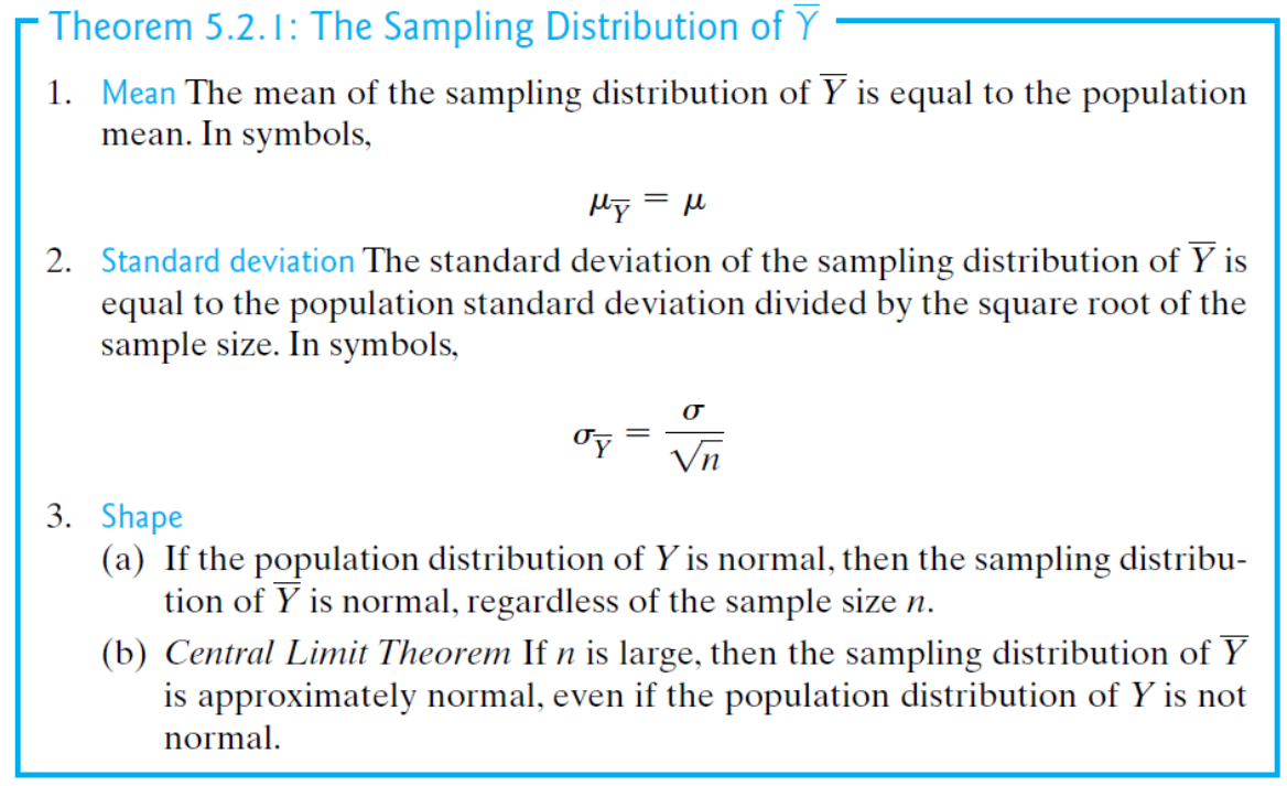
Let’s elaborate sampling distribution of \(\bar Y\).
Theorem 5.2.1
An Example
See Example 5.2.2 in our textbook.