
Assessing Normality
STAT 218 - Week 3, Lecture 4
January 25th, 2024
Today’s Agenda
Today, we will wrap up the week as follows:
recognize some summary statistics function in R
solve another probability exercise
assess normality
identify nonnormality and suggest some transformations
Standardization Formula
Remember!
- If a numeric variable has a continuous distribution, we can find probabilities by using the density curve for that variable.
- For that continuous variable, the probability would be equivalent to a specific area under the density curve.
- The area under a normal curve is always equals to 1.
- The calculated values for the potential areas under the normal curve are provided in Table 3.
- For that continuous variable, the probability would be equivalent to a specific area under the density curve.
Standard Normal Distribution
Standardization Formula
\(Z\) = (\(Y\) - \(\mu\)) / \(\sigma\)
Revisiting Tuesday’s Example
Please refer 4.3.1 from our course textbook.
Keep in mind that those are actually probability values.
Percentile
It is also possible to make an inverse reading of Table 3.
Let’s say we want to find the value on the Z scale that cuts off the top 2.5% of the distribution. Can you spot the number?
We often need to determine corresponding z-values when we want to determine a percentile of a normal distribution.
The percentiles of a distribution divide the distribution into 100 equal parts, just as the quartiles divide it into 4 equal parts.
Another example: We want to find the 70th percentile of a standard normal distribution.
Assessing Normality
Introduction
- We can assess normality by employing multiple strategies.
- The 68/95/99.7 Rule: We can check how closely a variable of Y conforms to a normal curve model.
The 68/95/99.7 Rule: We can check how closely a variable of Y conforms to a normal curve model.
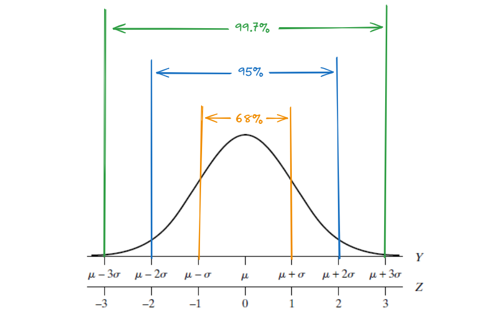
- See Example 4.4.1 and Example 4.4.2 from our textbook.
2 - Normal Quantile Plots
- Assessing the bell-shaped nature of a histogram visually can be challenging.
- The normal quantile plot was developed to overcome this challenge.
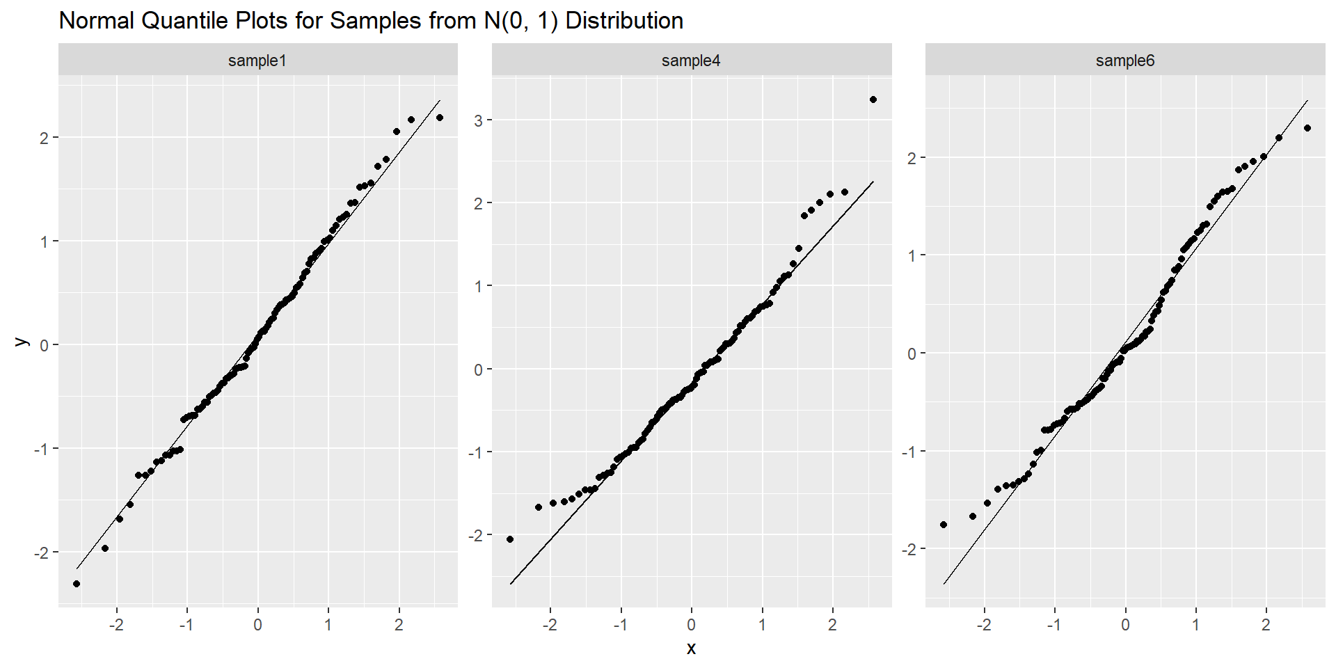
- I won’t go into theoretical plotting details, but the main idea is that a linear appearance in the plot suggests agreement between observed and theoretical values.
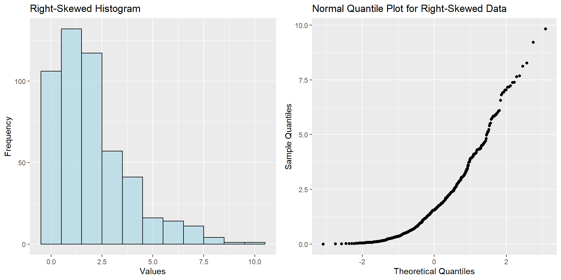
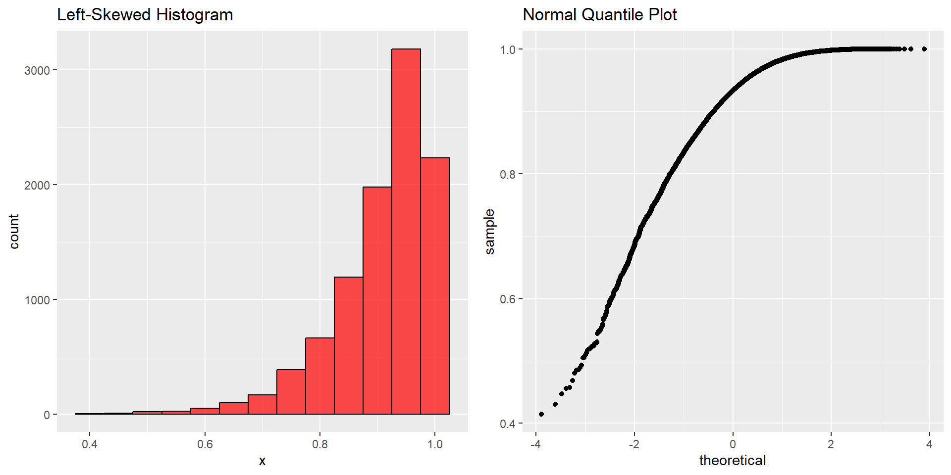
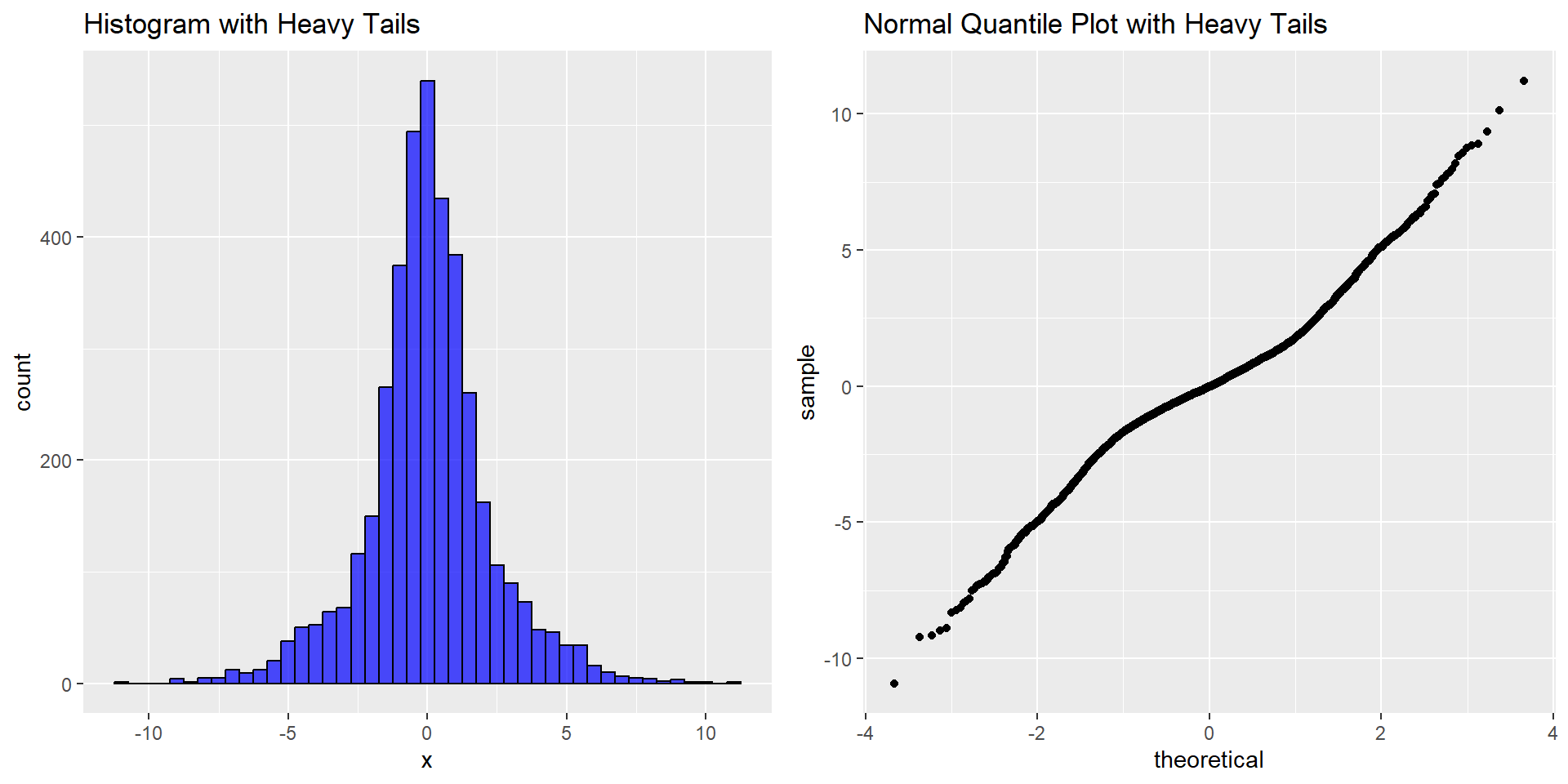
- If the data deviate from the normal model, the plot may exhibit strong nonlinear patterns, such as curvature or S shapes.
Normal Quantile Plots
Right-Skewed
Left-Skewed
Heavy Tails
Transformations
A Brief Introduction
Assessment with Normal Quantile Plot: Utilizing a normal quantile plot allows us to evaluate if the data originates from a normal distribution.
Identification of Non-Normality: Occasionally, both a histogram and normal quantile plot indicate non-normality in the data.
Transformation for Symmetry: Despite initial non-normality, transforming the data might yield a symmetric, bell-shaped curve.
Analysis in Transformed Scale: In such cases, it could be beneficial to proceed with the analysis in the newly transformed scale to better understand the underlying distribution.
Some Tips
- Skewed Right Distribution:
- Consider transformations like \((1/Y)\), \(\log(Y)\), \((1/\sqrt{Y}\) or \(\sqrt{Y}\).
- These transformations aim to mitigate the right-skewness, pulling in the long right-hand tail and extending the short left-hand tail for a more symmetric distribution.
- The choice of transformation depends on the severity of skewness, with more drastic transformations being considered for heavier skewness.
- Skewed Left Distribution:
- If the distribution of a variable \(Y\) is skewed to the left, raising \(Y\) to a power greater than 1 can be beneficial in addressing the left-skewness.
Shapiro-Wilk Test
Introduction
While normal quantile plots are preferred over histograms for visually assessing departures from normality, our perception remains subjective.
Shapiro–Wilk Test is a statistical method that provides a numerical assessment of evidence for certain types of nonnormality in data.
- The procedure’s mechanics are complex, but statistical software packages simplify the testing process.
Output and Interpretation:
- The output of the Shapiro–Wilk test includes a P-value.
- Interpretation:
- P-value < 0.001: Very strong evidence for nonnormality.
- P-value < 0.01: Strong evidence for nonnormality.
- P-value < 0.05: Moderate evidence for nonnormality.
- P-value < 0.10: Mild or weak evidence for nonnormality.
- P-value \(\geq 0.10\): No compelling evidence for nonnormality.