Descriptive Statistics in R

STAT 218 - Week 3, Lecture 3, Lab 2

January 24^th, 2024

Today’s Menu

Today we will be familiar with

• Data Frames
• Loading Data into R
• Summary Statistics
• ggplot()

Last Week’s Favourites - 1

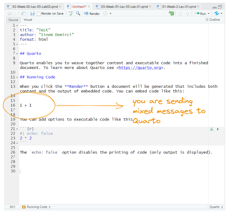
No boundaries

Last Week’s Favourites - 2

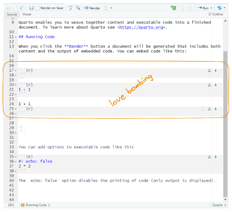
Quarto Loves Secure Attachment

How to Build A Healthy Relationship with Quarto

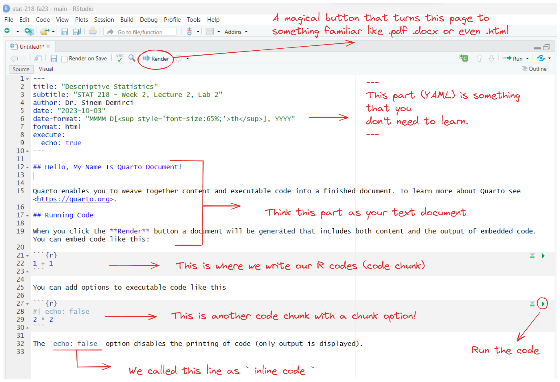
Quarto Document Parts

Before Proceeding Further…

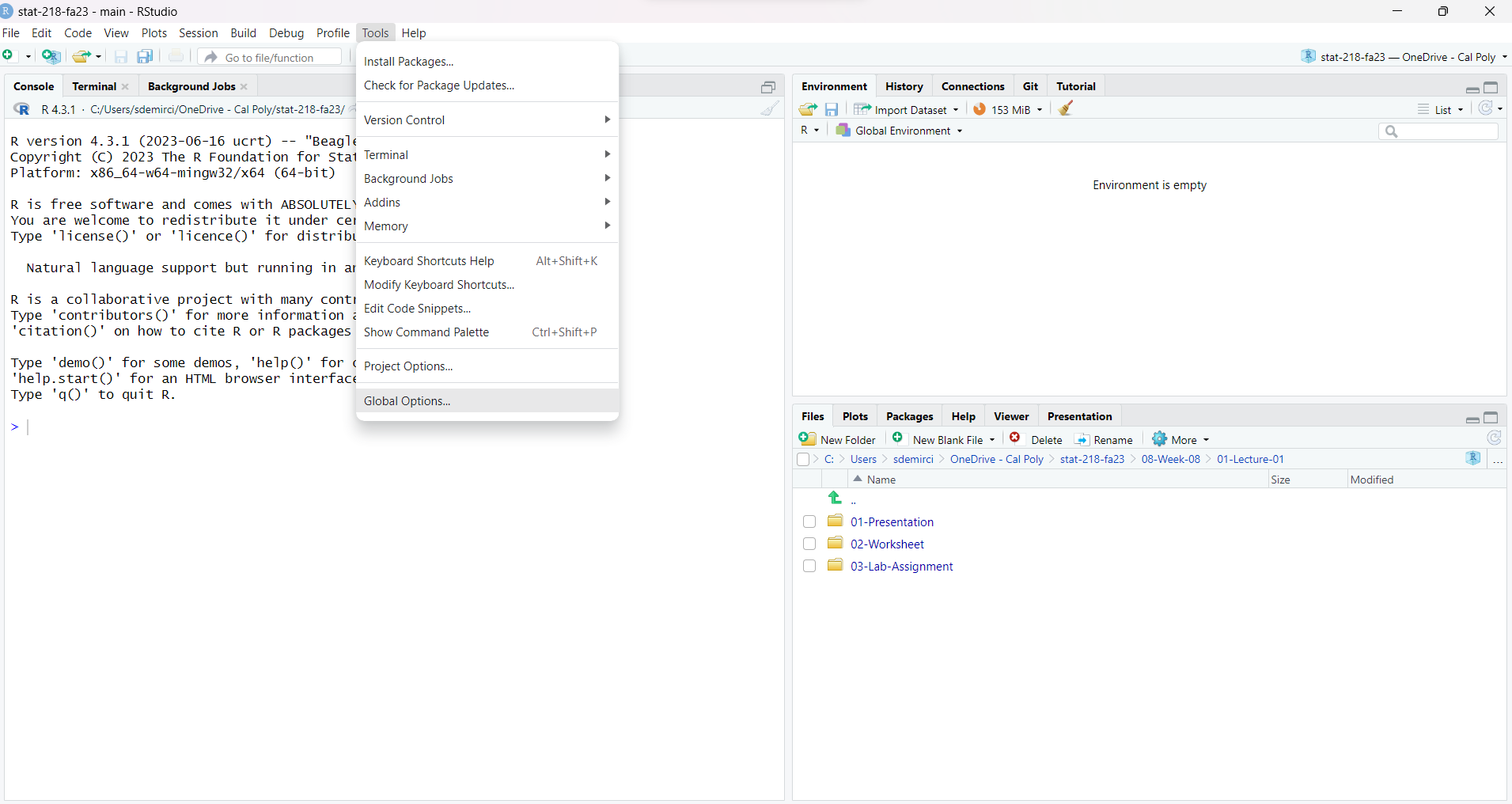
Before Proceeding Further…

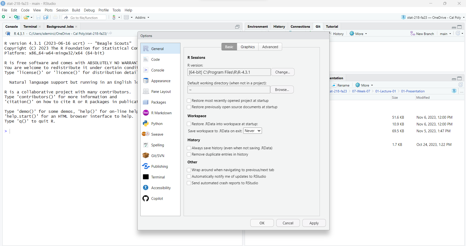
Creating This Week’s Quarto Document

Tip

• Let’s create this week’s Quarto document by clicking File > New File > Quarto Document
• Give a title as “Week 3 Lab 3 Descriptive Statistics”
  
• Add your own notes and the given codes to this document
  
• DO NOT FORGET to save it to your STAT 218 Folder!

Library Function in R

The library() function in R is like opening a toolbox. Imagine you have a toolbox filled with different tools, and each tool helps you do a specific job. Similarly, in R, a library is like a toolbox that contains specialized tools (packages) for specific tasks.

When you use the library() function, you’re telling R to open a specific toolbox (load a package) so that you can access and use the tools inside.

Let’s add a code chunk to our Quarto document and type the code below.

library(tidyverse)
library(openintro)

How to Load Data into R

We have two different ways to do that (within the scope of this class)

• Using an available dataset stored in R (packages)
• Importing a dataset from an outside source

Let’s use a dataset from openintro package.

data("births")

Import Dataset from An Outside Source

• We can import data from Text (.txt) or Excel (.csv OR .xls).

• Please download the dataset available on Canvas page titled as Data For Lab 3.

• SAVE THIS DATASET TO YOUR STAT218 FOLDER!

• Below, you see an example how to load data into R.

haircolordata <- read_csv("lab3data.csv")

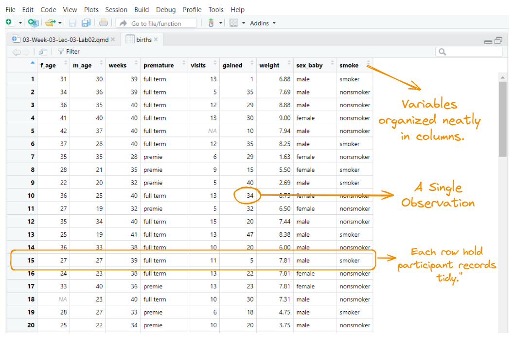
Getting to Know Your Data

After importing our data, it is important to familiarize with our data. We have some functions to do that.

Let’s start with glimpse() function. The name of this function is self-explanatory.

glimpse(haircolordata)

glimpse() function gives us a brief information about out data set. We have 6 variables and 180 cases or observations.

Getting to Know Your Data

Alternatively, we can ask R the number of columns (variables) and rows (cases) as following:

ncol(haircolordata) ## gives us the number of columns (variables)

[1] 6

nrow(haircolordata) ## gives us the number of rows (cases)

[1] 180

Assume that I would like to see just the names of the variables in my data set. I can use name()function for this.

names(haircolordata)

[1] "Hair"     "Birth"    "Handspan" "Siblings" "Shoes"    "Height"  

Frequency Distribution Table (An Ugly One!)

Let’s construct a frequency distribution table by using count()function.

count(haircolordata, Birth)

# A tibble: 12 × 2
   Birth         n
   <chr>     <int>
 1 April        14
 2 August       14
 3 December     19
 4 February      8
 5 January      15
 6 July         20
 7 June         11
 8 March        16
 9 May          11
10 November     15
11 October      18
12 September    19

Measures of Central Tendency

We can calculate measures of central tendency by using these unsurprising functions.

mean(haircolordata$Height)

[1] 172.8333

median(haircolordata$Height)

[1] 173

Measures of Central Tendency

Alternatively, you can use summarize() function for the same calculation.

summarize(haircolordata, mean(Height))

# A tibble: 1 × 1
  `mean(Height)`
           <dbl>
1           173.

summarize(haircolordata, median(Height))

# A tibble: 1 × 1
  `median(Height)`
             <dbl>
1              173

Measures of Dispersion

sd(haircolordata$Height) # sample standard deviation
var(haircolordata$Height) # sample variance

Alternatively, you can use summarize() function.

summarize(haircolordata, sd(Height))

# A tibble: 1 × 1
  `sd(Height)`
         <dbl>
1         8.96

summarize(haircolordata, var(Height))

# A tibble: 1 × 1
  `var(Height)`
          <dbl>
1          80.3

Or…

summarize(haircolordata,
          mean(Height),
          median(Height),
          sd(Height),
          var(Height))

# A tibble: 1 × 4
  `mean(Height)` `median(Height)` `sd(Height)` `var(Height)`
           <dbl>            <dbl>        <dbl>         <dbl>
1           173.              173         8.96          80.3

An Example for Bar Chart

Let’s plot a simple bar chart. Next session, we will explore other features for ggplot().

ggplot(data = haircolordata,
       aes(x = Hair,
           fill = Hair)) + 
  geom_bar(stat = "count") +
  labs(title = "Hair Color of Participants",
       x = "Hair Color",
       y = "Number of Participants"
       )

DO NOT FORGET TO SAVE THIS FILE IN YOUR STAT 218 FOLDER!