Chapter 4: The Normal Distribution
STAT 218 - Week 3, Lecture 2
January 23th, 2024
Notations
We will use some notations for important parameters and statistics as follows:
Important
Population Mean: \(\mu\)
Sample Mean: \(\bar{y}\)
Population Standard Deviation: \(\sigma\)
Sample Standard Deviation: \(s\)
Introduction to Normal Curves - I
- We can think of normal curves as a smooth approximation to a histogram based on a sample of \(Y\) values.
- We can describe the population distribution of a quantitative variable \(Y\) by
- calculating its mean \(\mu\) and its standard deviation \(\sigma\) AND
- using a density curve
- density curve: relative frequencies as areas under the curve.
- Let’s have a look at Example 4.1.2 in our book.
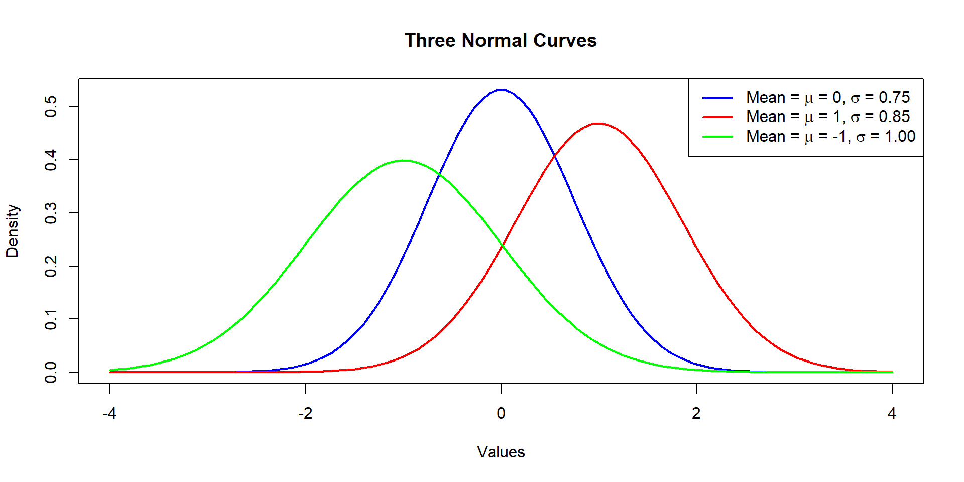
Introduction to Normal Curves - II
- There is no one single normal curve but many normal curves
- each normal curve has its own mean \(\mu\) and its standard deviation \(\sigma\)
Normal Curves, Continuous Variables and Probability
- If a numeric variable has a continuous distribution, we can find probabilities by using the density curve for that variable.
- For that continuous variable, the probability would be equivalent to a specific area under the density curve.
- The area under a normal curve is always equals to 1.
- Why?
- The area under a normal curve is always equals to 1.
- For that continuous variable, the probability would be equivalent to a specific area under the density curve.
Let’s Meet with Standard Normal Distribution
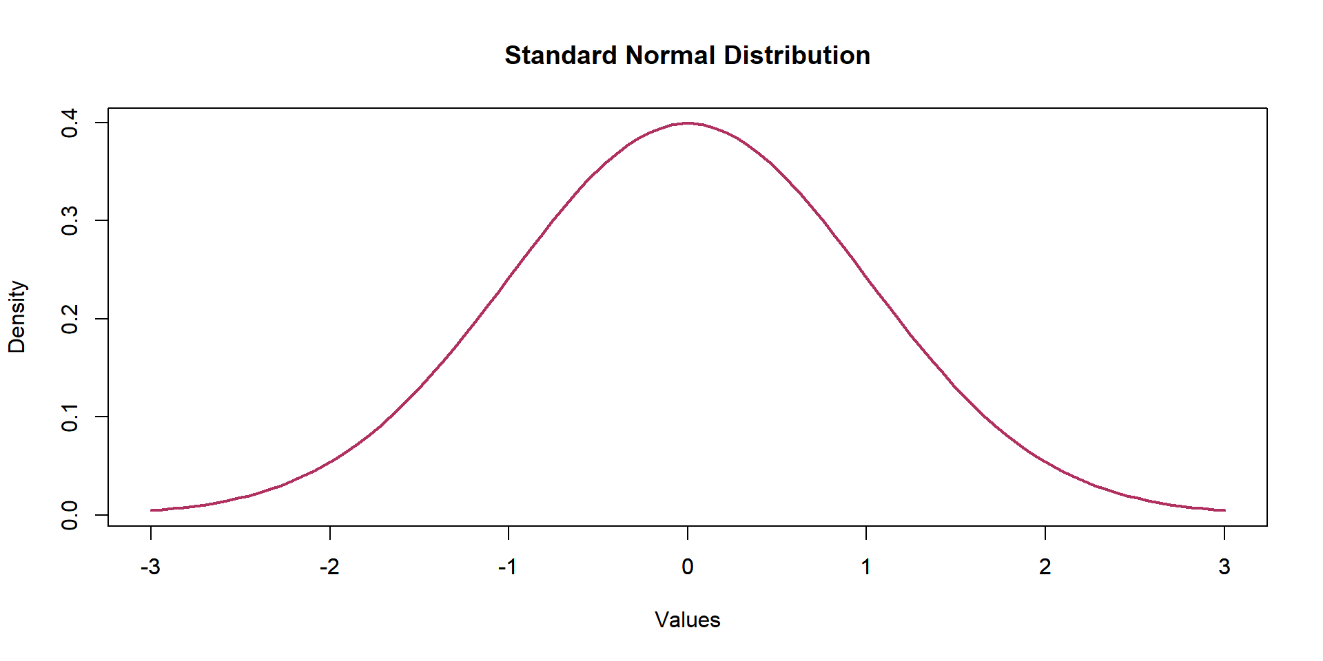
Standardization Formula
\(Z\) = (\(Y\) - \(\mu\)) / \(\sigma\)
Let’s See Examples
- Please refer Example 4.1.2 and 4.3.1 from our course textbook.
Review 2 - Quiz
See the ungraded Review 2 Quiz on Canvas (Module Week 3).
References
Samuels, M. L., Witmer, J. A., & Schaffner, A. A. (2003). Statistics for the life sciences (Vol. 4). Upper Saddle River, NJ: Prentice Hall.