Chapter 2: Description of Samples and Populations

STAT 218 - Week 2, Lecture 3

January 18^th, 2024

Let’s Refresh Our Memory

In the last 2 weeks, we

• discussed the differences among anectodal evidence, observational study, and experimental study
• defined the terms population and sample
• examined different types of random sampling
  
• had an introduction to descriptive statistics
  • saw some examples of frequency distributions enabling us to summarize categorical data and/or numeric data
    • either as a table or a graph

And OF COURSE

• We took our first steps in R!

What about Today?

Today we will see some examples to understand

• the shape, center, and dispersion in a data set.

More on Histograms

• A histogram is like a visual story in two parts.

  • Look at the tops of the bars to understand the distribution’s shape.
  • The area within each bar tells us two things:
    • It is proportional to the corresponding frequency.
    • It represents the number of observations in that category.

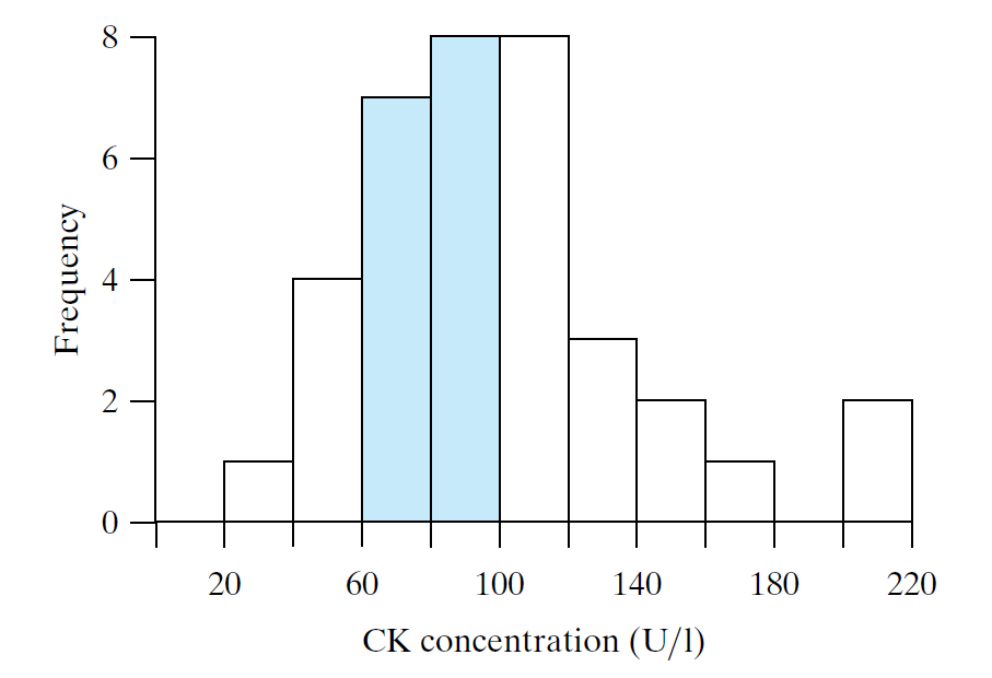
• Let’s elaborate yesterday’s example

  • The shaded area is 42% of the total area in all the bars.

• 42% of the CK values fall into the corresponding classes
• 15 out of 36 values lie between 60 U/I and 100 U/l.

Shapes of Distributions

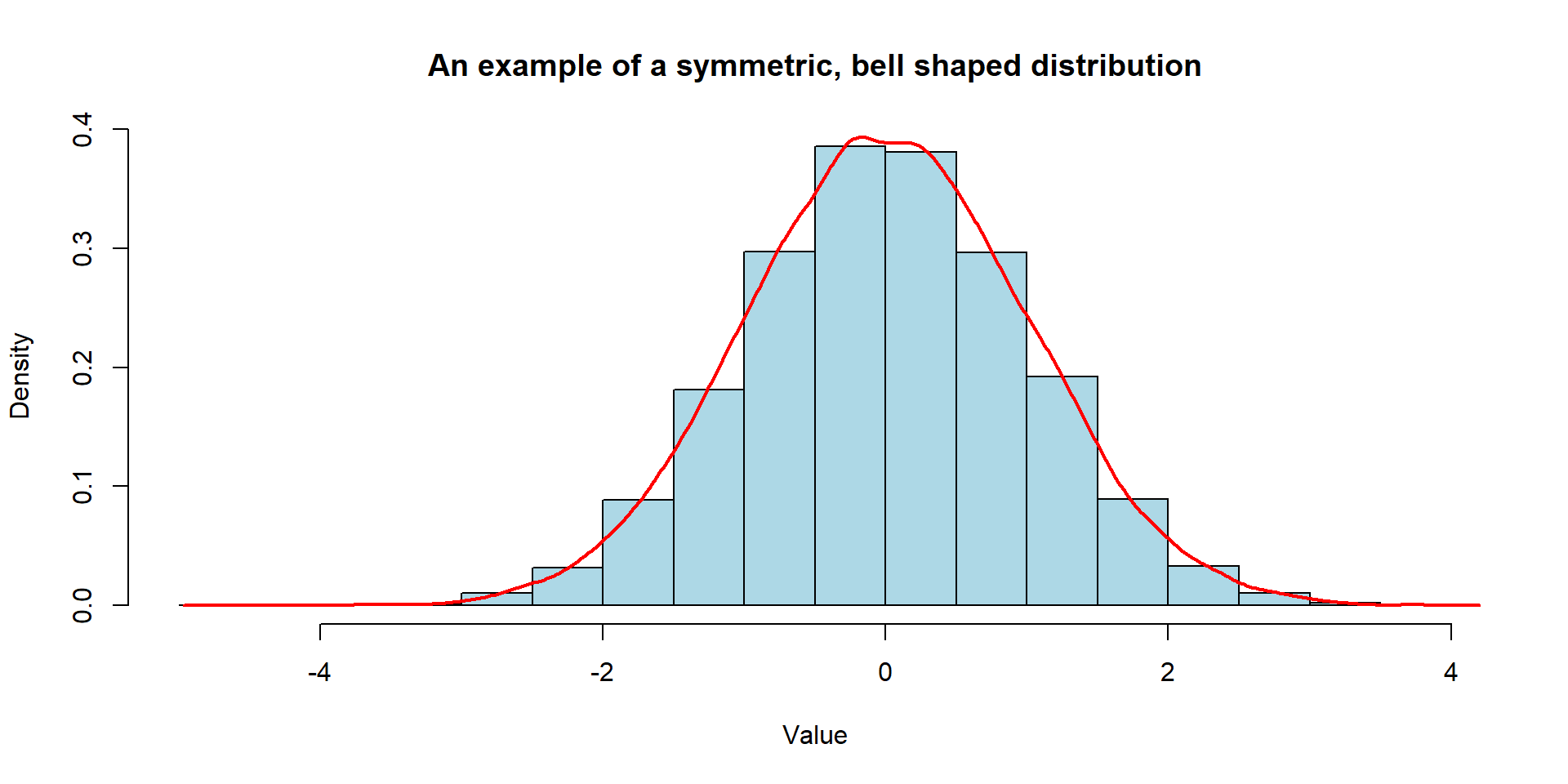
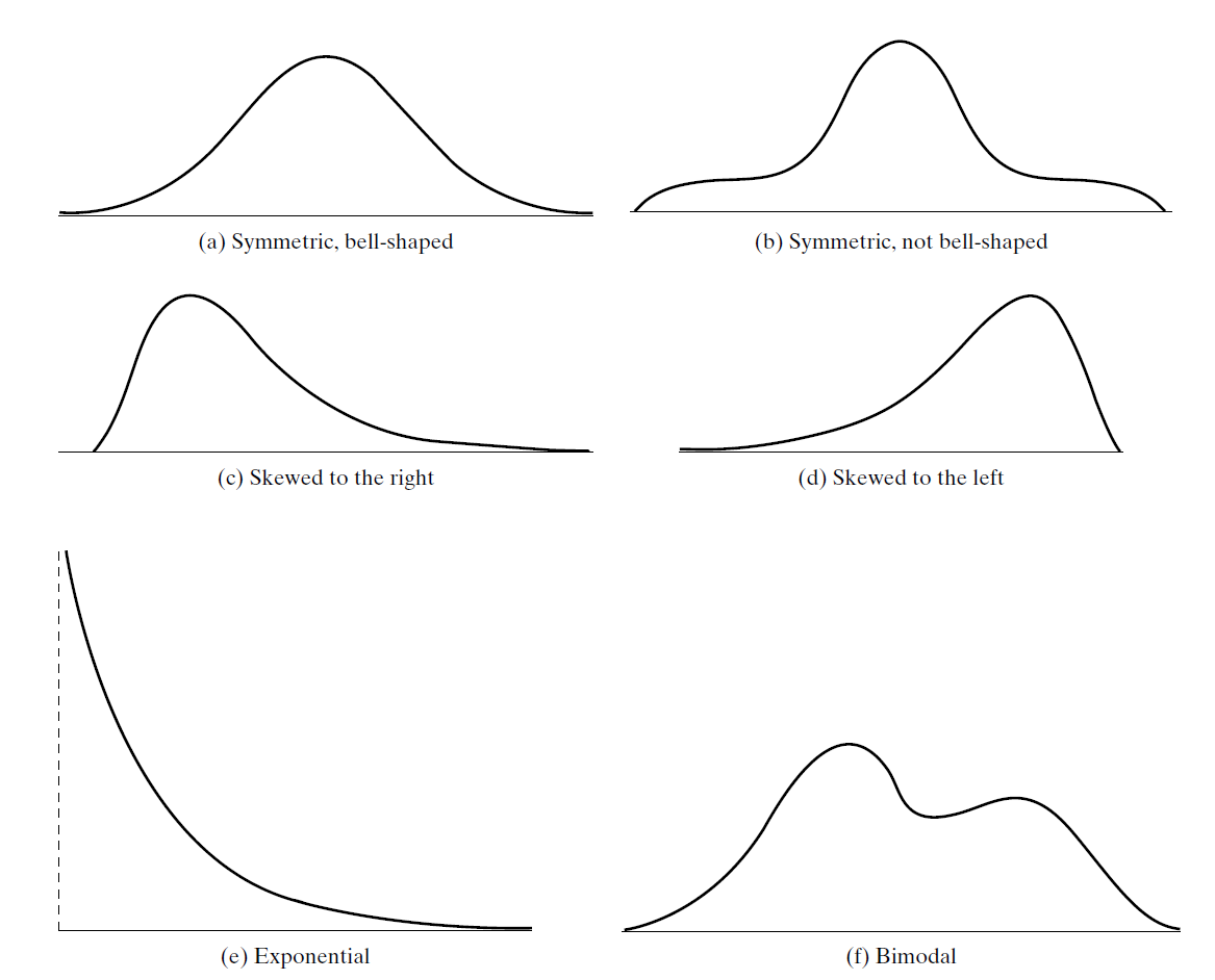
The shape of a distribution can be represented by a smooth curve that provides an approximation of the histogram.

Shapes of Distributions

Central Tendency

Measures of Center

To understand the center or typical value of a data set, we calculate

• Mean
• Median
• Mode

We also call these as “Central Tendency”

Mean

• You might be familiar with this term. It is also known as
  • arithmetic mean OR sample mean

Tip

Remember we employed a symbolic convention to differentiate between a variable and an observed value of that variable.

• \(Y = birthweight\) (Variable)
• \(y = 12.8\) lb (Observed Value)

We now denote

• the observations in a sample by \(y_1\), \(y_2\), . . . , \(y_n\)
• the mean of the sample by the symbol \(\bar{y}\) (read “y-bar”).

Mean

We calculate the mean by using this formula

Median

• Imagine what would happen if Bill Gates was in our class and we calculated the average money in our bank account.
  • It might not be the best idea to interpret this average.
• Instead, we can calculate median which is a value that splits the ordered data into two equal parts.

How to Find the Median

• Arrange the observations in increasing order.
• In the array of ordered observations, the median is
  • the middle value (if n is odd) or
  • midway between the two middle values (if n is even).
• We denote the median of the sample by the symbol \(\tilde{y}\) (read “y-tilde”).

Mode

• The mode in a dataset is the number that occurs with the highest frequency.
• It serves as a measure of central tendency, indicating the most prevalent choice or the characteristic that appears most frequently in your sample.

Let’s have another toy example

• Assume that we have a following dataset:
  • 22, 6, 6, 4, 2

Measures of Center	Data and Calculation	Result
Mean	(2+4+6+6+22)/5	8
Median	2,4,6,6,22	6
Mode	2,4,6,6,22	6

Robustness

• A statistic is said to be robust if the value of the statistic is relatively unaffected by changes in a small portion of the data, even if the changes are dramatic ones.
• The median is a robust statistic, but the mean is not robust because it can be greatly shifted by changes in even one observation.

Mean vs. Median

• Both are useful measures!

Warning

• Mean value is related to the sum which makes it sometimes very little sense.
  • In some situations in life science such as bioassay, survival, and toxicity studies, the mean value cannot be computed (until last patient has died, for instance) whereas the median can be calculated.

• Median is more robust than the mean.
  • Remember Bill Gates example!
• Mean can be sometimes more efficient than median.
  • Mean takes full advantage of all the information available which makes it a rock star in classical methods in statistics.

Visualizing Mean and Median

• Let’s see Rossman & Chance Applet to visualize mean and median.

Spread of Distributions

Let’s assume we managed to collect data from our squirrels on campus :) Our class was divided into three groups, and each group measured the weights (lbs) of 10 squirrels. Here are the results:

Group 1: 1.25, 1.25, 1.25, 1.25, 1.25, 1.25, 1.25, 1.25, 1.25, 1.25

Group 2: 1.0, 1.0, 1.0, 1.0, 1.0, 1.5, 1.5, 1.5, 1.5, 1.5

Group 3: 1.0, 1.4, 1.2, 1.4, 1.1, 1.3, 1.6, 1.0, 1.2, 1.3

Dr. Demirci mentioned that looking at these numbers is so confusing. Can you please calculate the sample mean for them to summarize this data?

All these groups calculated the same mean, which is 1.25 lbs. Dr. Demirci seemed not so happy with this number.

• Why?

Spread of Distribution

• So far, we’ve explored the shapes and central tendencies of distributions
  • but an effective depiction of a distribution should also capture its dispersion
    • whether the observations in the sample are mostly uniform or exhibit significant variation.
• We can also report this by using
  • Range
  • Standard Deviation
  • Interquartile Range

Range

• Range is one of the measures of dispersion indicating the difference between largest and smallest observations in a sample.

• Let’s calculate range

  • Group 1: \(1.25 - 1.25 = 0\)
  • Group 2: \(1.5 - 1.0 = 0.5\)
  • Group 3: \(1.6 - 1.0 = 0.6\)

Warning

• Range is easy to calculate, but very sensitive to extreme values
  • It is not robust.

Standard Deviation and Variance

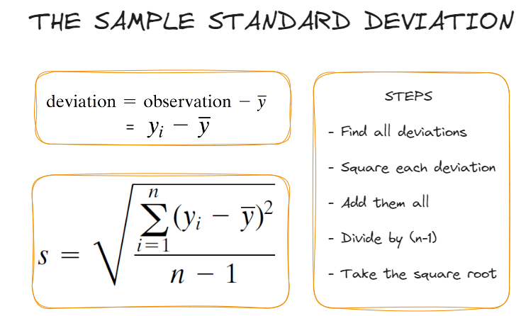
• Variance is denoted as \(s^2\), which is the standard deviation squared
• Let’s calculate standard deviation for each squirrel group!

Quartile Range & Interquartile Range

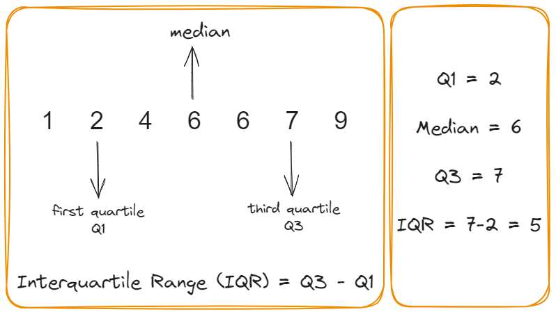
Comparison of Measures of Dispersion

• The range is simple to understand, but it can be a poor descriptive measure because it depends only on the extreme tails of the distribution.
  • highly nonrobust.
• The interquartile range, by contrast, describes the spread in the central “body” of the distribution.
• The standard deviation takes account of all the observations and can roughly be interpreted in terms of the spread of the observations around their mean.
  • However, the SD can be inflated by observations in the extreme tails.
• The interquartile range is a robust measure, while the SD is not robust.